Upernavik, NW Greenland New Islands, Nunataks and Former Glacier Base Exposed

On May 30, 2017April 28, 2024 By mspeltoIn Greenland glacier retreat

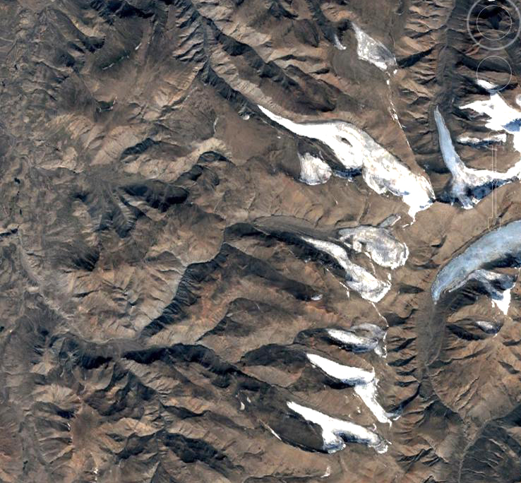
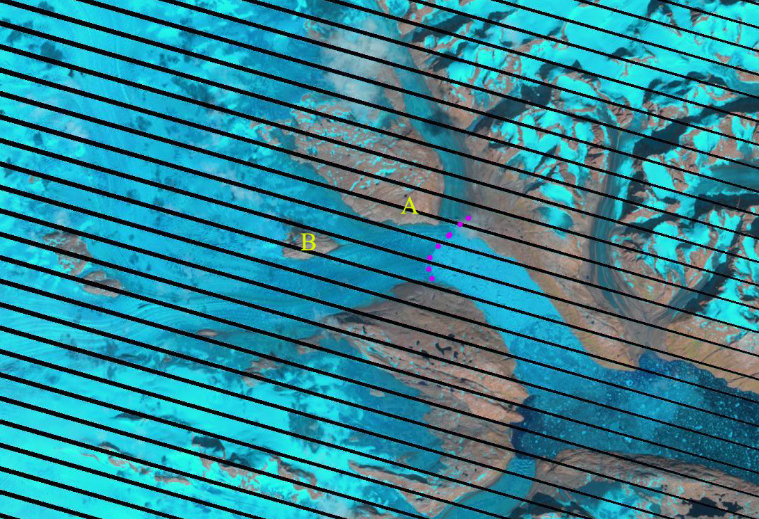
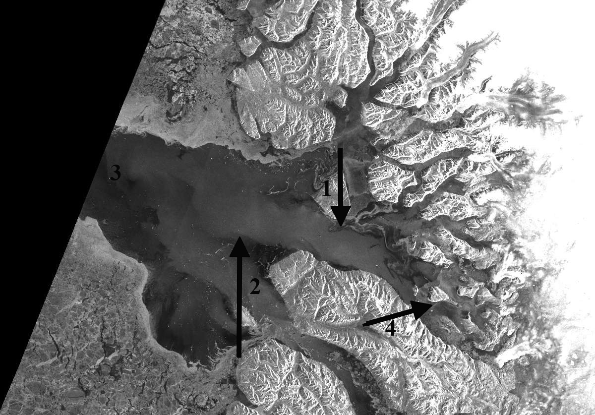
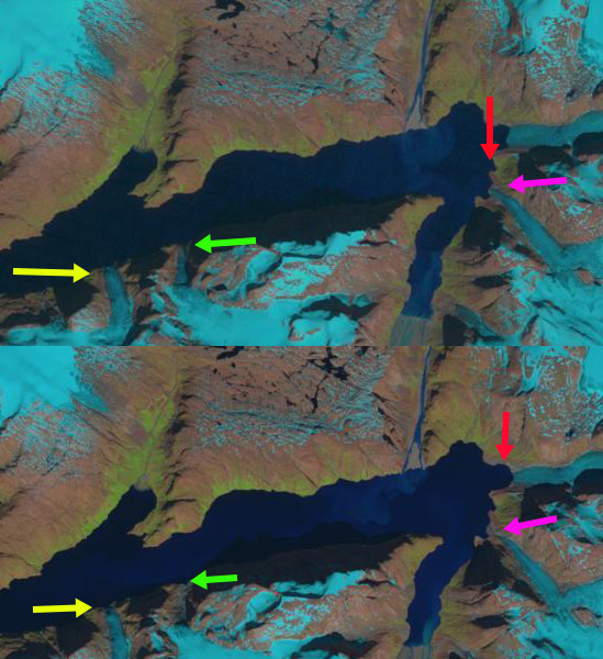
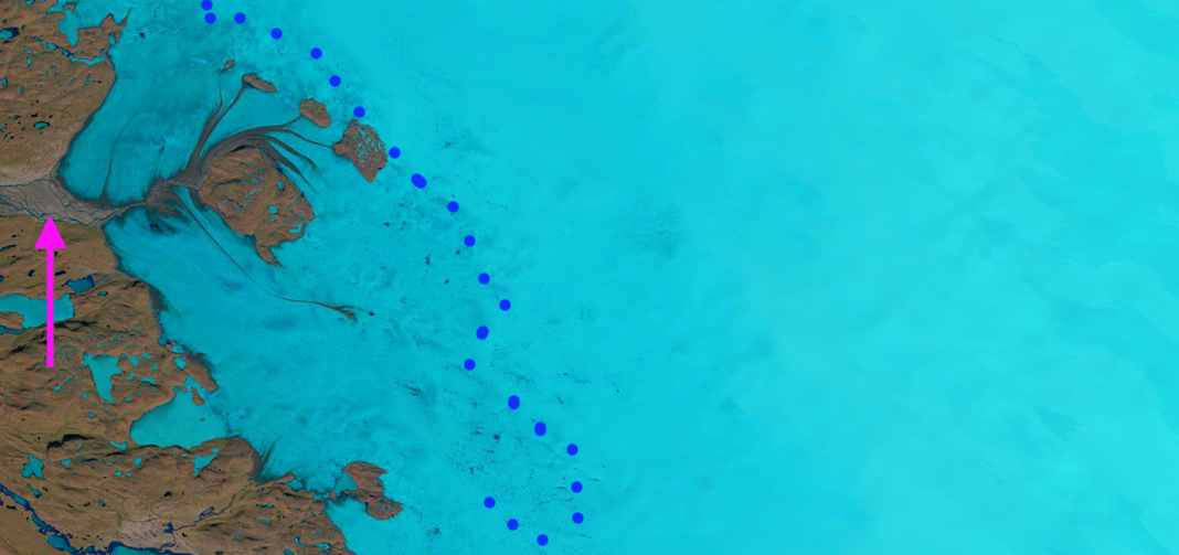
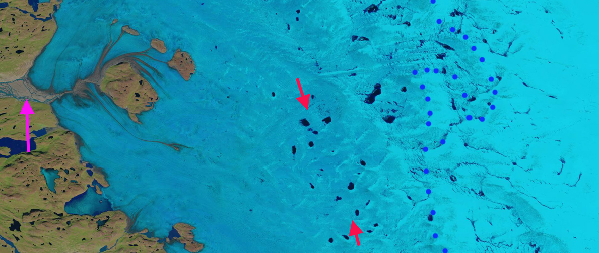
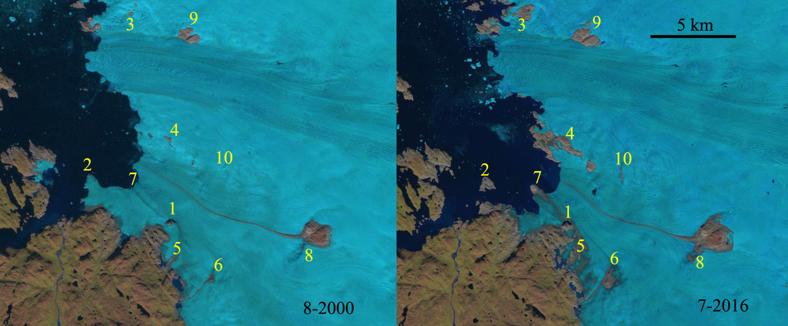
Upernavik Glacier in Landsat images from August 2000 and August 2016. Each Point is at the same location in both image, and the changes are noted in the discussion below. The same locations are also identified in the July 2001 and Aug. 2016 image below.

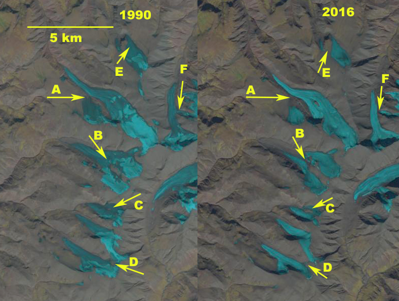
Upernavik Glacier is on the NW Greenland Coast the next major outlet north of Rinks Glacier. Today the glacier has four separate main calving termini, that was a single terminus until 1980. The retreat of this glacier is exposing new islands, nunataks etc that is examined in Landsat images from 2000 to 2016. Howat and Eddy (2011) observed the terminus change of 71 outlet glaciers in NW Greenland from 2000-2010 and found that 98% had retreated. The retreat has occurred irrespective of the different characteristics of various glaciers (Bailey and Pelto, SkS). Box and Decker (2011) note that ice loss for Upernavik Glacier’s combined termini was 7.9 square kilometers per year from 2000-2010. Larsen et al (2016) observed asynchronous changes in dynamic behavior of four outlets of Upernavik between 1992 and 2013. Velocities were stable for all outlets at between 1992 and 2005. The northernmost glacier began acceleration and thinning in 2006 -2011. The second most northerly outlet began acceleration and thinning in 2009 and this continued through at least 2013. The southern glaciers showed little change. They observed that the southernmost which is the focus here underwent a small deceleration between 1992 and 2013. Velocity data for the 1999-2014 period of the southernmost outlet is available using an online map browser (Rosenau et al; 2015), indicates the highest velocity of the southernmost branch occurred in 2013 and 2014, which would also lead to enhanced thinning. Moon et al (2014) observed the velocity of the southernmost arm of Upernavik to have a velocity of 2-3 km per year with a modest seasonal velocity fluctuation of ~15%. They note that Upernavik Glacier is a type 2 glacier, exhibiting relatively stable velocity from late summer through winter into spring, followed by a strong early summer speedup and midsummer slow down.

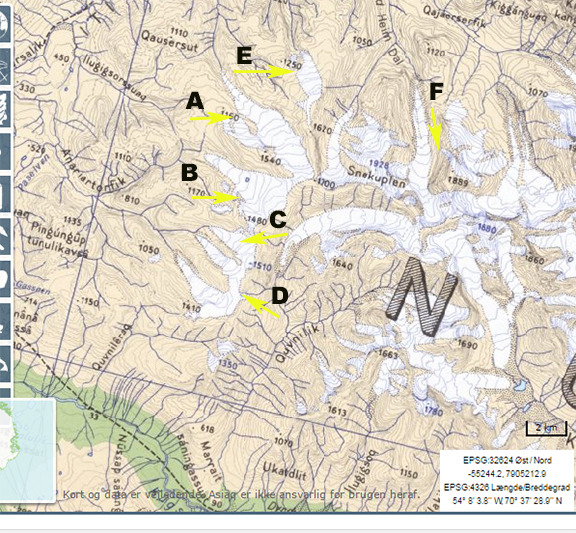
Here we examine the changes from 2000 to 2016 at ten locations near the front of the southern most of the main outlets of Upernavik Glacier. This reveals the formation of new islands, exposure of the former glacier bed and expansion of nunataks.

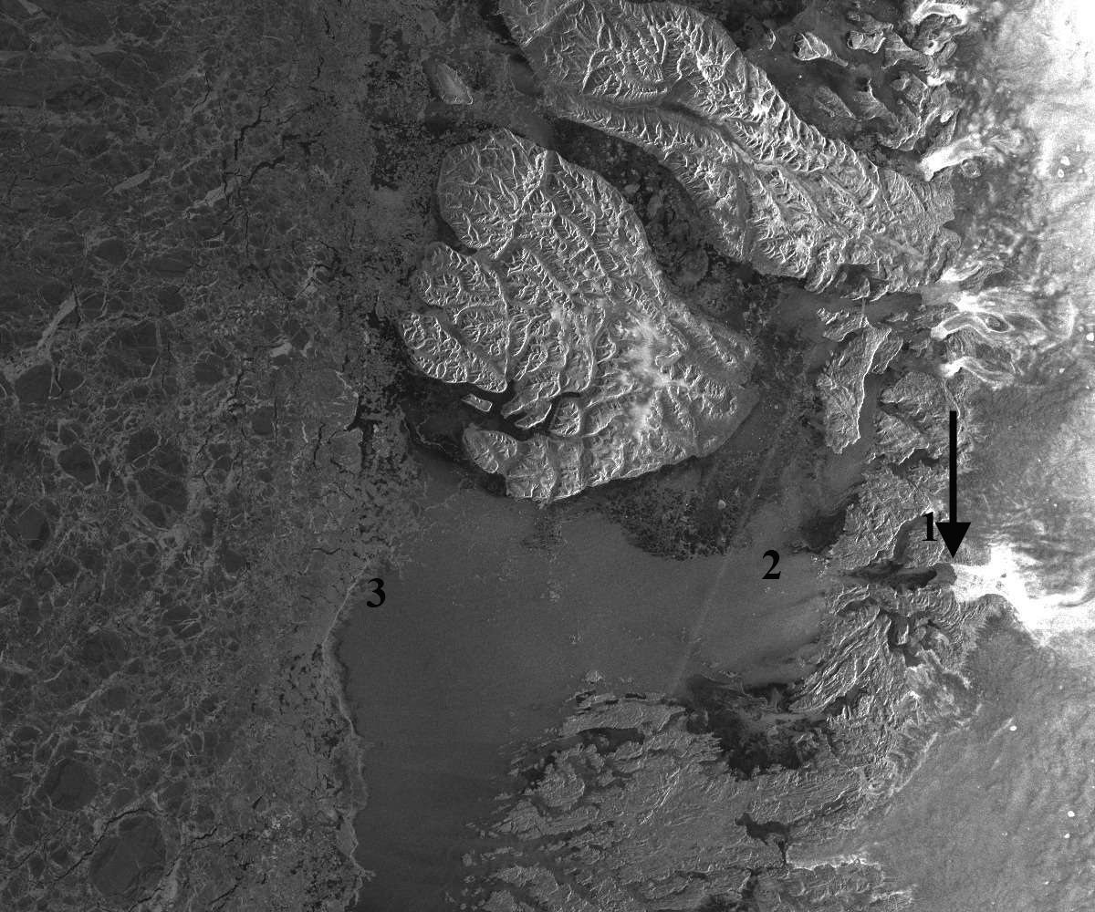
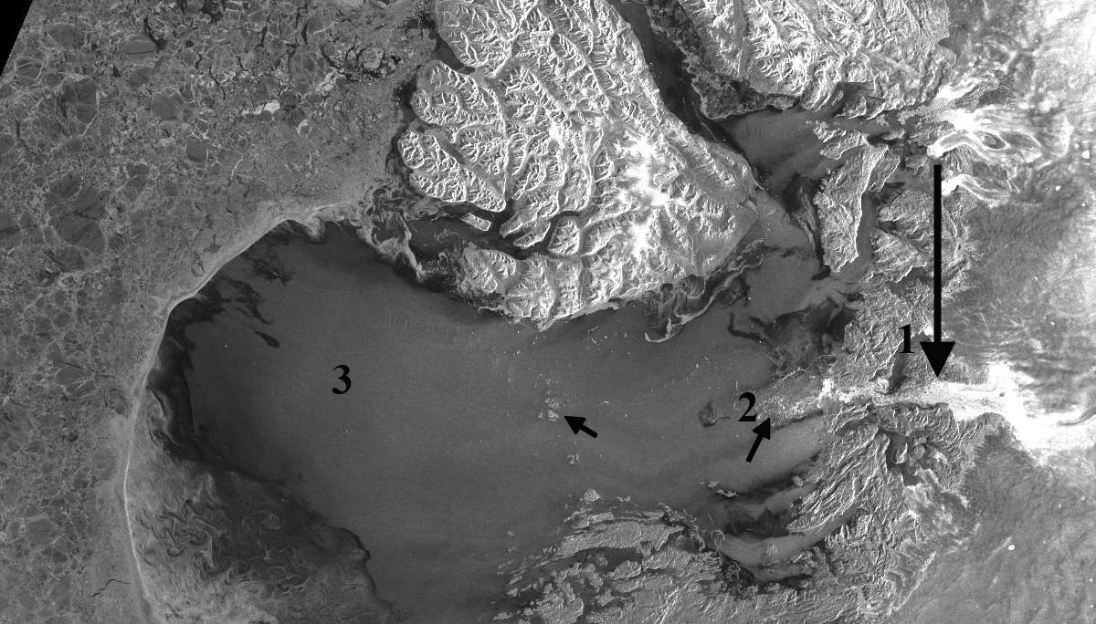
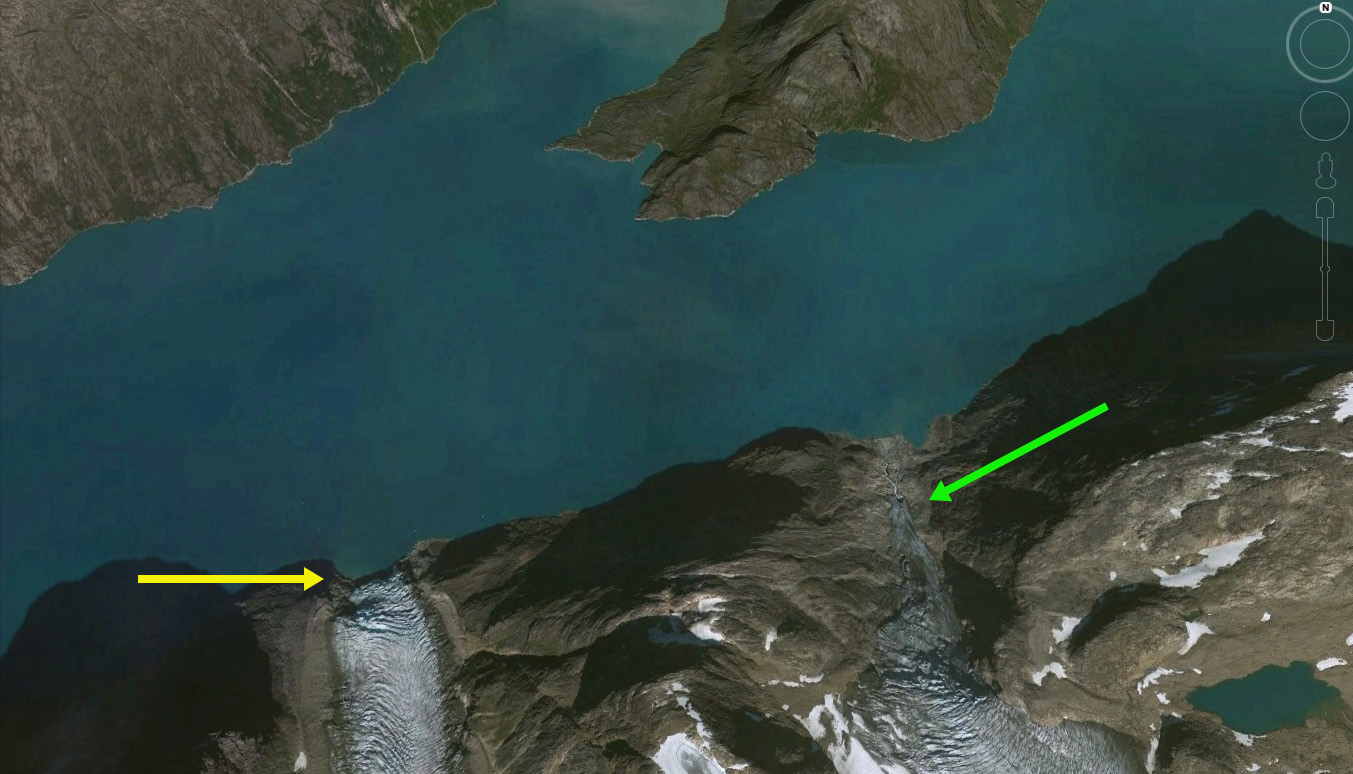
Point 1: In 2000 and 2001 this is a nunatak just below the number that is separated by 500 m of glacier from the edge of the ice sheet. In 2016 this point is a knob at the edge of the glacier.

Point 2: This is an area of bedrock, just below the number where the glacier terminates in 2000 and 2001. In 2016 this is an island that is 2.5 km from the ice front.

Point 3: In 2000 and 2001 this indicates a small area of bedrock just above the number, that is less than 300 m across. In 2016 this is a large area of bedrock that is over 1 km across and is merging with other bedrock areas near the glacier front.

Point 4: Is a small area of bedrock just west of the number that is 2 km from the ice front in 2000 and 2001. In 2016 this area of bedrock has merged with bedrock at the terminus of glacier and extends 3 km from the ice front inland.

Point 5. This is a region surround the number that is under ice in 2000 and 2001, there is a narrow rib of rock extending from the edge of the glacier to Point 5. In 2016 a large area of the former glacier bed is exposed with numerous streamlined bedrock features.

Point 6 is a small area of bedrock in 2000 and 2001 that is 2 km from the glacier edge. In 2016 this has become an area that extends 1 km from north to south and has a narrow bedrock connection to the glacier edge. The former glacier bed will continue to be expose between Point 5 and Point 6.

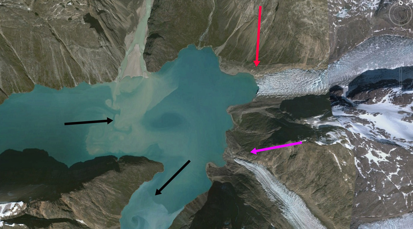
Point 7: In 2000 and 2001 this point marks the ice front where a medial moraine reaches the terminus. In 2016 this is an area of bedrock that will either become a new island or merge with bedrock at Point 1.

Point 8: Just west of the number in 2000 and 2001 is a single small outcrop of bedrock less than 200 m across. In 2016 the area of bedrock extends south for 1 km from the main nunatak that is also expanding.

Point 9: In 2000 and 2001 this location is covered by ice 500 m north of a nunatak. In 2016 a new bedrock knob has emerged that will soon join the main nunatak.

Point 10: In 2000 and 2001 this location is covered by ice 5 km from the ice front. In 2016 a one kilometer long bedrock rib has emerged due to glacier thinning.

The retreat of this glacier exposing new islands and nunataks is repeated at Steenstrup Glacier, Alison Gletscher and Kong Oscar Glacier

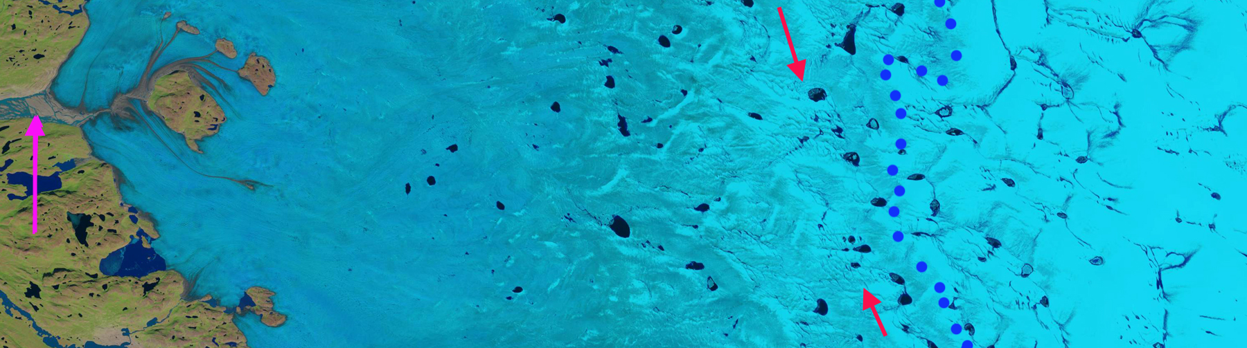
Upernavik Glacier in Landsat images fromJuly 2001 and Aug. 2016. Each Point is at the same location in both image, and the changes are noted in the discussion above.

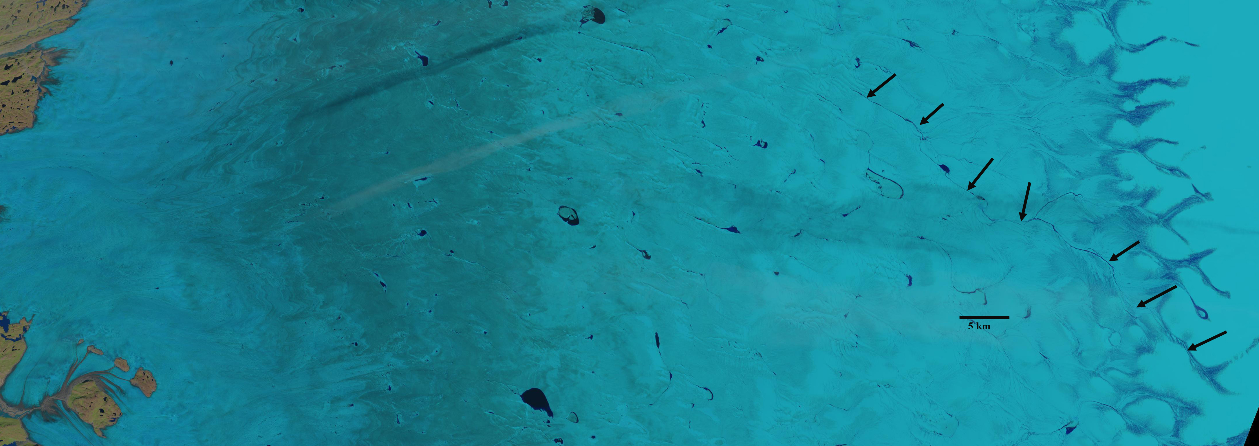
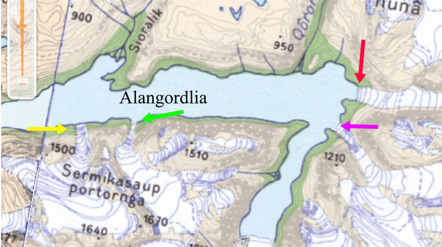
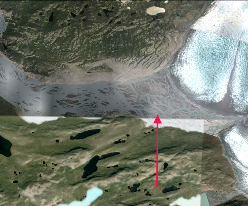
View of the Upernavik four main calving fronts. The focus here is on what is deemed the south trunk. This is from the University of Dresden velocity map portal.

Nuusuaq Peninsula West Greenland Glacier Disintegration

On April 19, 2017May 1, 2024 By mspeltoIn climate change glacier retreat, Greenland glacier retreat

Comparison of alpine glaciers on Nuussuaq Peninsula in 1990 and 2016 Landsat images. Each arrow is at a specific location in both images exhibiting glacier separation/disintegration.

The Nuussuaq Peninsula is just north of Disko Island in West Greenland and is home to many alpine glaciers and small ice caps. Here we examine the furthest west group of alpine glaciers on the peninsula. This group is 125 km west of the ice sheet and is not influenced directly by the ice sheet, but instead is most sensitive to the conditions over the Davis Strait and Baffin Bay just 25 km away. The glaciers are near Snokpulen Peak, 1928 m. Smaller ice caps around the Greenland Ice Sheet have been losing mass. Citterio et al (2011) documented the existence of 1172 glacier in 2001 on Disko Island, Nuussuaq Peninsula and Svartenhuk Peninsula. West Greenland. Bolch et al (2013) using Landsat imagery and ICESat altimetry data noted that peripheral ice caps and glacier provided a significant fraction,~14 or 20% of the reported overall mass loss of Greenland to sea level. This is equivalent to 10% of the estimated contribution from the world’s alpine glaciers and ice caps to sea level rise. Noël et al, (2017) observed that in ~1997 a tipping point for the peripheral ice caps/alpine glaciers of Greenland occurred in terms of mass balance. The onset of a rapid deterioration in the capacity of the glaciers firn to refreeze meltwater led to mass losses and consequent glacier runoff increased 65% faster than meltwater production. Mittivakkat Glacier is an example of this trend.

Here we compare 1990-2016 Landsat images indicating the changes in the alpine glaciers near Snokpulen Peak. At Point A,B,D and F there is a glacier connection between tributaries or adjacent glaciers. At Point C and E there is an area of limited bare ground amidst the glacier. Also notice in 1990 there is retained snowpack on the glaciers. In the 2002 image below there is also retained snowpack. In 2016 there is not retained snowpack on the glaciers, indicating the lack of an accumulation zone. Without an accumulation zone there is not firn for meltwater to percolate into and refreeze. Meltwater is then not recaptured and is lost as noted by Noël et al, (2017), to be a widespread occurrence. The adjacent glaciers at Point A, B, D and F are now separated. The extent of bare ground near point C and E has expanded significantly. The area loss here underscores the volume loss of the peripheral ice caps that Bolch et al (2013) observed.

2002 Landsat image indicating some retained snowpack on the glaciers.

Topographic Map of the region on Nuussuaq Peninsula.

Google Earth image of region, indicating the separation/disintegration that is occurring.

A River Runs 40 km Across the Greenland Ice Sheet

On February 27, 2017May 1, 2024 By mspeltoIn glacier climate change, Glacier Observations, Greenland glacier retreat

Supraglacial stream, on July 26, 2016 Landsat image, stretching 40 km across the ice sheet from the transient snowline, which marks the boundary between the percolation zone and the wet snow zone, west toward the ice sheet margin, note black arrows.

The Greenland Ice Sheet has experienced a significant increase in surface melt. This is due both to warmer temperatures and enhanced melt due to a reduction in reflectivity-albedo. The expansion in melt area, duration and intensity (NSIDC, 2015) has also generated large volume of meltwater transported via supraglacial streams. Recent work by Tedesco et al (2016) and Kintisch et al (2017) illustrate three key reasons for the albedo change in the melt zone.

1) Upon melting and refreezing, ice crystals lose their branched shape, grow larger and rounder, which reduces the reflectivity of the snow by as much as 10%.

2) Satellite data show that the margins of the ice sheet have darkened by as much as 5% per decade since 2001. Dust trapped over the centuries has become concentrated at the melting edge of the ice sheet.

3) The combination of algae and bacteria with dust generates a sludge—known as cryoconite. This dark material gathers in depressions decreasing albedo. Black and Bloom is a project focused on how dark particles (black) and microbial processes (bloom) darken and accelerate the melting of the Greenland Ice Sheet

Tedesco et al (2016) noted the negative trend in albedo is confined to the regions of the ice sheet that experience summer melting. They also observed no trend during the 1981–1996 period. Their analysis indicates the albedo decrease is due to the combined effects of increased air temperatures, which enhances melt promoting growth in snow grain size and the expansion of bare ice areas, and to increasing concentration of dark impurities on ice surfaces. Kintisch et al (2017) noted the same mechanisms with warmer summers also enhancing microbes and algae growth on the wetter surface of the ice, producing more cryocontie, that reduces albedo absorbing more solar energy. Cryoconite is more spatially limited than the other mechanisms. They also observed that soot and dust that blow in from lower latitudes and darken the ice are also increasing.

The darker surface enhances melt which generates more meltwater largely drained in the melt zone by supraglacial streams. Smith et al (2015) documented the surface drainage in the ablation zone of the southwest GIS. They focused on documenting the distribution of over 500 high order stream channel networks in a 6812 square kilometer region, inland from Kangerlussuaq. All of the stream networks terminated in moulins before the ice sheet edge (NASA, 2015). This indicates that moulins are common, important and sparse.

Poinar et al (2015) observe the longest streams in the 30-50 km range. Here we examine two streams one in detail using Google Earth that is 30 km long and a 40 km long surface stream in 2016 observed in Sentinel 2 and Landsat images. That the surface rivers can travel this distance across the surface before draining via a moulin indicates that the glacier is not structurally like Swiss cheese (Pelto, 2015). The Google Earth detailed view illustrates both the darker surface, the maturity and hydrologic efficiency of the thermally incised meltwater streams.

The stream observed in Google Earth in its mid-reach has an average of 15 m in width. The slope of the ice sheet is 1/120 in this region, with the river beginning at 1320 m and ending at 1070 m. Gleason et al (2016) examined numerous supraglacial streams and noted that supraglacial streams with a width of 15-20 m and slopes of 1/100 to 1/200 had a depth of 1.5-2.0 m and velocity of ~0.5 m/sec. This suggests the stream here has a discharge of 7-10 cubic meters per second. The darkness of the ice surface indicating a low albedo is also apparent. The ice is not nearly as dark when standing directly on it as it is in the macro-scale.

[ngg_images source=”galleries” container_ids=”52″ display_type=”photocrati-nextgen_basic_imagebrowser” ajax_pagination=”1″ template=”/nas/wp/www/sites/blogsorg/wp-content/plugins/nextgen-gallery/products/photocrati_nextgen/modules/ngglegacy/view/imagebrowser-caption.php” order_by=”sortorder” order_direction=”ASC” returns=”included” maximum_entity_count=”500″]

The second stream is seen in a Sentinel image from July 15 and a Landsat image from July 26. The black arrow indicate the stream that is 40 km long. The stream extends from 110 km from the edge of the ice sheet to within 75 km. The stream begins near the transient snowline at 1650 m and ends near 1400 m, creating a slushy valley above the local percolation zone. The stream in early July flows through the wet snow zone. By the end of the July the lower section of the stream becomes a bare ice region, the upper remains in the wet snow zone.

Supraglacial stream in mid-July Sentinel images stretching 40 km across the ice sheet from the transient snowline west toward the ice sheet margin.

Norrearm Fjord Glacier Retreat, Greenland

On December 9, 2016May 1, 2024 By mspeltoIn glacier climate change, Glacier Observations, Greenland glacier retreat

Apostelens Glacier in Norrearm Fjord Landsat comparison from 1999 to 2016. Red arrows are the 1999 terminus location, yellow arrows the 2016 terminus location and purple arrows indicate an expanding bedrock ridge.

“Apostelens” Glacier drains east from a peak of the same name into an arm of Norrearm Fjord, which in turn is part of Lindenow Fjord in southern Greenland. The glacier is a short distance north of Kangersuneq Qingordleq, where recent retreat has led to glacier separation. The glacier is soon to lose its tidewater connection as has occurred at Tasermiut Fjord to the west. This will result in a decline in iceberg production as well.

Here we examine Landsat imagery from 1999-2016 to identify glacier change. In 1999 the Apostelens arm of Norrearm Fjord is largely filled by the glacier which extends to within 2.5 km of Norrearm Fjord, red arrow. The tongue contains numerous ogives formed each year due to seasonal velocity changes through an icefall. This is evident in the Google Earth image from 2004, where 24 ogives are evident on the low slope glacier tongue, in 1999 the number is over 30. By 2013 the glacier has retreated nearly 2 km from the 1999 terminus position, red arrow. In 2012 Google Earth imagery indicates increased crevassing near the front and the loss of most ogives. New ogive formation is also hard to distinguish. By 2016 the glacier has retreated 2.6 km and is nearing the headward limit of the fjord arm. The collapse of the fjord tongue and its associated ogives indicates the loss of 30 years worth of volume flux that emerged from the icefall that generated the ogives.

Greenland tidewater outlet glaciers in this region have experienced substantial retreat since 1990, Weidick et al (2012) and Howat and Eddy (2011). Murray et al (2015) examined 199 tidewater glaciers in Greenland and noted significant retreat of 188 of them. Apostelens Glacier was not one of these, and soon will not be a tidewater glacier to be included in the list.

Apostelens Glacier in Norrearm Fjord Google Earth comparison from 2004 and 2012. Red arrows are the 2004 terminus location, and yellow arrows the 2012 terminus location. Note ogives in 2004 and loss of them in 2012.

Map of the Norrearm Fjord region and Apostelens Glacier, with blue arrows indicating flow.

Tasermiut Fjord, Greenland loses its Glacier Connection

On October 21, 2016May 1, 2024 By mspeltoIn glacier climate change, Glacier Observations, Greenland glacier retreat1 Comment

Landsat image sequence from 1999-2016. Red arrows mark the 1999 terminus, yellow arrows the 2016 terminus and the purple arrow a tributary that detaches from Semitsiaq (S). Tasermiut Sermeq (T) retreats from the fjord.

Tasermuit Fjord in southern Greenland is noted for its beauty, and until recently the fjord terminated at a glacier front. Currently no glacier reaches to the fjord. The retreat over the last two decades is similar to neighboring glaciers Kangersuneq Qingordleq and Qaleriq. The loss of direct glacier connection is also occurring at Alangordlia. Here we examine Landsat images from 1999-2016 to observe glacier change. At the head of the fjord is Sermeq Tasermiut and on the east side is Sermitsiaq.

In 1999 the Sermitsiaq Glacier terminated at the eastern end of a small lake, red arrow. Tasermiut Sermeq terminated in the fjord, red arrow. By 2002 Sermitsiaq had retreated from the lake, while Tasermiut Sermeq still reached the fjord. In 2013 Tasermiut Sermeq had retreated from the fjord and Sermitsiaq had retreated substantially from the lake and also had a significant tributary from the north detach, purple arrow. In 2016 Sermitsiaq has retreated 700 m since 1999, yellow arrow. Biggs (2011) had noted a 610 m retreat of the glacier from 1987-2009, a slower rate than since 1999. Tasermiut Sermeq has retreated 300 m since 1999,and has a narrow steep tongue that will melt back quickly in the near future.

Murray et al (2015) examined 199 tidewater glaciers in Greenland and noted significant retreat of 188 of them. This is changing fjord dynamics, which will in the case of Tasermiut affect the marine biology, which has not been studied in any detail yet. Students on Ice 2014 Arctic Expedition provides exceptional imagery of this fjord and the Nanotarlik region.

Google Earth imagery of the region. illustrating the loss of fjord connection after 2009.

Map of the region

Kangersuneq Qingordleq, Greenland Retreat Causes Separation

On October 18, 2016May 1, 2024 By mspeltoIn Greenland glacier retreat

Landsat comparison from 1999, 2001, 2013 and 2016 of Kangersuneq Qingordleq. Red arrow is 1999 terminus, yellow arrow is 2016 terminus. Purple dots mark the transient snowline and the purple arrow a detached tributary.

Kangersuneq Qingordleq is one of the most southerly tidewater glaciers in Greenland. It is a 15 km long glacier flowing from the mountains between Prince Christian Sound and Lindenow Fjord. It is more akin to an Alaskan tidewater outlet glacier than ice sheet fed Greenland outlet glaciers. Greenland tidewater outlet glaciers in this region have experienced substantial retreat since 1990, Weidick et al (2012) and Howat and Eddy (2011). Howat and Eddy (2011) examined 200 tidewater glaciers in Greenland from 2000 and 2010 observing that 191 had retreated, rapid retreat was observed in all sectors of the ice sheet. Moon and Joughin (2008) observed a synchronous ice sheet–wide increase in tidewater retreat from 2000–2006 versus 1992–2000, coincident with a 1.1°C increase in mean summer temperature. There was also an increased in sea surface temperature (Straneo et al, 2013). The retreat of glaciers in southern Greenland is changing the physical geography and hence physical oceanography of the fjords.

Here we examine Landsat imagery from 1999-2016 to identify recent behavior. In 1999 the glacier terminated at a narrow point in the fjord, red arrow. This location is also just beyond a junction with a tributary from the east. The fjord was just 600 m wide which would act as a pinning point restricting calving. It would not be surprising if fjord depth was also reduced here. By 2001 the glacier has retreated a short distance from the narrow point and is beginning to separate from the tributary. The transient snow line is at 950-1000 m. By 2005 the glacier had retreated 800 m and had fully separated from the eastern tributary, the ice front was 1 km wide. By 2013 the glacier has retreated into a section of the fjord that is 1.2 km wide and the transient snowline is at again at 950-1000 m. By 2016 the glacier has retreated 2.8 km since 1999. The transient snowline is 1000-1050 m in 2016, which is high enough to drive continued retreat. The fjord further widens to 1.4 km, 2.5 km behind the glacier front. This suggests that retreat will continue as there will be less sidewall stabilization. The glacier since 1999 has lost nearly 20% of its total length. To the northeast Qaleraliq has experienced a 3.2 km of its west arm and 1.2 km of its east arm from 1992 to 2012. To the northeast Tingmiarmiit Glacier retreat from 1999-2015 has led to complete separation of the western and northern tributary. The western tributary is the main glacier and has retreated 2.4 km and the northern tributary has retreated 2.2 km in the 16 year period. In the case of nearby Tasermiut Fjord retreat has led to fjord losing its tidewater connection.

Terminus of Kangersuneq Qingordleq in 2005 Google Earth image. Red arrow is 1999 terminus, yellow arrow is 2016 terminus.

Map of the region around Kangersuneq Qingordleq. Red arrow is 1999 terminus, yellow arrow is 2016 terminus.

Moulins: Clarifying Impacts on Glacier Velocity

On September 1, 2016September 2, 2016 By mspeltoIn glacier climate change, Glacier Observations, Greenland glacier retreat

In the last week I have read three separate articles referring to glacier moulins as lubricating the bed of a glacier resulting in overall velocity increase, for example EOS (Aug. 2016), this is not generally accurate. Having spent considerable time observing moulins and reviewing some excellent studies that indicate their impact, it is worth noting again a more complete picture of the role moulins play. This is a role that warrants considerable further examination. In 2008 and 2011 I wrote a piece indicating why this a generalization that is only sometimes accurate. The key to increasing glacier velocity is high basal water pressure, not simply lots of meltwater. Think of your car, if you have low oil pressure that is an issue for efficient running. If you have high oil pressure that is ideal. If you have high oil pressure and you add more oil that does not further lubricate the engine. Delivering more water to the base of a glacier that already has lots of meltwater drainage will not typically lead to a significant acceleration. A number of studies since 2008 have better illustrated this principle as it applies to ice sheets.

Ahlstrøm et al (2013) examined 17 Greenland glaciers and noted a pattern, “Common to all the observed glacier velocity records is a pronounced seasonal variation, with an early melt season maximum generally followed by a rapid mid-melt season deceleration”. This indicates the Greenland glaciers are more like a typical alpine glacier and are susceptible to the forces that tend to cause alpine glaciers to experience peak flow during spring and early summer. Those forces are the delivery of meltwater to the base of the glacier, when a basal conduit system is poorly developed. This leads to high basal water pressure, which enhances sliding. As the conduit system develops/evolves the basal water pressure declines as does basal sliding, even with more meltwater runoff.

This is what has been reported to be the case by Sundal et al (2011) in Greenland. They found a similar early season velocity in all years, with a reduced velocity late in summer during the warmest years. This suggested that a more efficient melt drainage system had developed, reducing basal water pressure for a longer period of time. The meltwater lubrication mechanism is real, but as observed is limited both in time and area impacted. It is likely that, as on alpine glaciers, the seasonal speedup is offset by a greater slowdown late in the melt season. Most observed acceleration due to high meltwater input has been on the order of several weeks, leading to a 10-20% flow increase for that period.

Moon et al (2014) examined 55 Greenland glaciers and found three distinct seasonal velocity patterns. Type 1 behavior is characterized by speedup between late spring and early summer with speed remaining high until late winter or early spring, with the principal sensitivity being to terminus conditions and position. Type 2 behavior has stable velocity from late summer through spring, with a strong early summer speedup as runoff increases and midsummer slowing, as the glacier develops an efficient drainage system. Type 3 behavior has a mid-summer slowdown leading to a pronounced late summer minimum during the period of maximum runoff. Velocity than rebounds over the winter. The common behavior is then a slowdown during periods of peak runoff and moulin drainage.

Anderson et al (2011) noted that changes in velocity due to a 45% change in meltwater input were small 4-5% on Helheim Glacier.

Clason et al (2015) modelled development of moulins and their ability to deliver the water to the bed of Leverett Glacier. This study illustrates the level of details that is being examined to better model meltwater routing, which will inform flow models as noted by EOS (2015).

Moulins increase meltwater flow to a glacier bed. In areas where significant surface melt occurs, this tends to lead to an early melt season increase in basal water pressure and then velocity. This is typically followed by a mid/late melt season deceleration with continued meltwater drainage through moulins. The lubrication is hence, restricted in time, and if followed by a deceleration, does not necessarily lead to an increase in the overall glacier velocity. Certainly in some cases moulins will increase overall velocity and in others not.

Tingmiarmit Glacier Retreat Separates Tributaries, South East Greenland

On May 30, 2016May 2, 2024 By mspeltoIn glacier climate change, Glacier Observations, Greenland glacier retreat

Tingmiarmit Glacier comparison in 1999 and 2015 Landsat images indicating the separation of tributaries at the terminus. The red arrows indicate the 1999 terminus and the yellow arrows the 2015 terminus location. Point A is peninsula where the tributaries joined, and Point B is a nunatak just upglacier from the 2015 terminus.

Tingmiarmit Glacier (Timmiarmiit also) ends in the Tingmiarmit Kangertivat Fjord in southeast Greenland. The glacier is just south of Heimdal Glacier and is noted by Rignot et al (2012) as having a velocity of 1.4 to 3 km/year. Moon et al (2012) note that most glaciers in SE Greenland experienced a significant velocity increase after 2000. In 1999 the glacier terminus was beyond the junction of two main tributaries, with little variation from 1994. Here we examine 1999-2015 imagery to identify the separation and retreat. The retreat is similar to that of nearby Thrym Glacier, which also had a tributary separation and nearby Puisortoq.

In 1999 the glacier terminates 1 km beyond the junction of the two tributaries, indicated by red arrow on each image. The fjord is 2.2 km wide at this point. The terminus had not changed in 2001 Landsat imagery. By 2010 terminus is now located at the junction of the two glaciers. which still share a single calving front, though the calving front is longer with northern and western facing section. In 2015 retreat has led to complete separation of the western and northern tributary. The western tributary is the main glacier and has retreated 2.4 km and the northern tributary has retreated 2.2 km in the sixteen year period. The retreat of the northern tributary has been slower since 2010. The western tributary now terminates 1.5 km from former junction.The fjord is expanding in width, which suggests the current terminus is not at a stable location. The nunatak marked B is a potential point of stability but not likely as the main arm of the glacier goes south of this location and then the fjord continues to expand. Moon and Joughin (2008) observed an ice sheet tidewater glacier retreat rate increase from 2000-2006, coinciding with an increase here. Howat and Eddy (2010) noted a mean change for this region of -107 m per year. Tingmiarmit Glacier’s rate of retreat was slightly higher at 120 m/year for the 1999-2010 period and . Polar Portal continues to expand the number of glaciers with updated terminus positions from satellite imagery with 20 presently.

Mountain Photographer Jack Brauer captured an excellent image of the terminus area in late August, particularly given it was out a commercial airliner window. This image illustrates the steeper slopes and much smaller contribution of the tributaries to the right (east) of Point A and B. The image also indicates that Point B is likely not a significant pinning point to stabilize the terminus. The map below from the Greenland Geological Data viewer indicates the change with the tributaries now disconnected.

Image from Jack Brauer, looking northwest toward Tingmiarmit.

Greenland Geological Data, from the Geological Survey of Denmark and Greenland.

2001 Landsat image

2010 Landsat image, purple dots indicate ice front.

What is Up in Disko-Uummannaq Bay Greenland January 9-16, 2016

On January 17, 2016May 2, 2024 By mspeltoIn Glacier Observations, Greenland glacier retreat5 Comments

@TenneyNaumer contacted Alun Hubbard, Jason Box and I with an astute observation last evening. “But what I am getting at is that in general the temperature anomalies over the region of Jakobshavn have been high in the last few days, and I spotted weird temperatures off the coast via Climate Reanalyzer (which is seriously low resolution). I just checked with the manati satellite (also seriously low resolution), and it seems some sort of event has taken place.”

Following up on what are typically good observations from Tenney I looked at the Radarsat-2 and Sentinel-1 imagery posted by the Danish Meteorological Institute. Weather records from automatic weather stations in the region from PROMICE and the surface mass balance model results for the week from Polar Portal.

It is evident from the PROMICE weather records on the ice sheet just south of the Disko Bay region that temperatures have been exceptionally high since January 5th and atmospheric pressures have been high since January 9th. The Polar Portal mass balance model indicates some actual declines/ablation in the last week. This is more likely sublimation from föehn conditions than actual melt. The real changes are in the sea ice fronts and ice in the coastal inlets illustrated by MODIS. Below are images from January 9, 11, 13 and 16 for Disko Bay and January 9, 13 and 16 from Uummannaq Bay.

The arrow at location 1# is an area of sea ice across the fjord in front of Jakobshavn Glacier on January 9, that disappears by January 13. Location #2 is at the fjord mouth and location #3 is at the sea front south of Disko Island on January 9. There is no real cloud cover evident in any of images. Maybe low level fog in places. By January 11th a plume is sweeping from Point 2 towards Point 3. Notice the sea ice in the fjord disappears by January 13th and the ice front is pushed back in a concave fashion at Point #3. This indicates a clear push of water driving sea ice offshore. The Ilulissat Fjord mouth lack of ice is also evident in Webcam images from 1-16-16 and 1-17-16 at the Hotel Arctic, last images below with two boats plying the open water. on the 16th and icebergs clogging the fjord mouth on the 17th. The Sentinel-1 image from January 16th shows a significant flushing of icebergs from Ilulissat Fjord, pointed out by black arrows. This image has better clarity and with the icebergs scattered through the plume, indicate more clearly the plume is a water source change event, even if wind driven. The iceberg plume in the fjord has a brighter aspect due to the varied surface aspect-reflectance and has expanded down fjord. The event must be due to or enhanced by strong offshore winds and Ruth Mottram (@ruth_mottram) indicates there was at least one föehn event this week. The plume includes bergs from the ice melange in front of Jakobshavn has been largely removed, which can have implications for calving and frontal velocity. Moon et al, (2015). indicate the role that a rigid ice melange has on the calving and frontal velocity of tidewater outlet glaciers in Greenland.

In Uummannaq Bay a very similar sequence plays out, note on January 9 the sea ice connecting islands near #4. By January 13th the ice at location #4 is gone. The ice front is now at location #3, which on January 9th was well into the ice pack. Again we have a clear push of water leading to a concave sea ice front that is pushed well offshore. Icebergs can be seen amidst plume on January 16th, the plume opacity and size has diminished since January 13th.

In both of the January 13th images there is a plume leading to the concave sea ice front, the question being is this sediment laden water, with the resultant higher reflectivity or is it a combination of a surface water change from wind or a combination. We had questioned if the plume had any sediment origin initially. Its widespread nature and persistence suggested not. Aeration was another suggestion. Jason Box suggests that the opaque water plume leading to the developing polyna is driven by the strong offshore winds and the opaque whitening is capillary waves on the sea surface. Examples of identification of observed high backscatter from offshore winds are from Monaldo and Beal (1998) and Li et al, (2007) The ice must in part be driven back by a surface water push. You can see icebergs in sections of the plumes closer to shore suggesting this is a surface near surface phenomenon. This is a short term event. However, it could have broader implications, in this case the ice melange in front of Jakobshavn has been removed, and probably from in front of other glaciers, which will impact near term calving rates. I have incorporated many insights from the community and welcome more.

RADARSAT-2 IMAGE FROM Disko Bay 1/09/2016

RADARSAT-2 IMAGE FROM Disko Bay 1/11/2016

RADARSAT-2 IMAGE FROM Disko Bay 1/13/2016

Sentinel-1 imagery from 1-16-16 of Disko Bay-notice expanded brightness area in the fjord by #1.

Sentinel 1 imagery of Uummannaq Bay 1/09/2016

RADARSAT-2 IMAGE FROM Uummannaq Bay MODIS 1/13/2016

Sentinel 1 imagery of Uummannaq Bay 1/13/2016 plume size and opacity diminishing.

Ilulissat Fjord mouth webcam view 1-16-16.

Ilulissat Fjord mouth webcam view 1-17-16.

Orpissuup Tasia Glacier slowdown, SW Greenland

On December 30, 2015May 2, 2024 By mspeltoIn climate change glacier retreat, glacier climate change, Greenland glacier retreat

Tedstone et al (2015) Figure 3 illustrates the widespread velocity decline along three transects.

Pelto et al (1989) after a field campaign we mounted in 1985 and 1986 on Jakobshavns Glacier noted that the velocity was essentially the same in the summer of 1964, 1976, 1978, 1985 and 1986. Further we observed that the agreement between surface mass-balance and volume-flux calculations, suggested that “Jakobshavns Isbrae: is almost in a state of equilibrium”. The point of the study was to establish a baseline of velocity before the anticipated acceleration due to warming. This acceleration due to warming happened beginning in 1992 from 20 m/day at the calving front in 1985 to 46 m/day in 2012, comparing the same locations the annual speed increase was 282% from 1992 to 2012 (Joughin et al 2014). The Jakobshavns Isbrae is a tidewater glacier, just south of the glacier the margin of the ice sheet is dominated by a land terminating section that has a different dynamic response to warming.

Tedstone et al (2015) in a paper published in Nature in October noted a decadal reduction in glacier velocity for a land terminating region of the Greenland Ice Sheet. This slow down occurred despite a 50% increase in meltwater production. This is emphasized in the figure above indicating the changes along three transects from green earlier to purple later years. A glacier inhabits a particular topographic environment that establishes the basic flow field. Climate change can affect glacier flow by increasing ice melt, which leads to ice thinning and a consequent reduction in force generating ice deformation and flow. This same ice melt can deliver meltwater to the base of the ice sheet, which can lead to short term increases in basal water pressure that will drive acceleration, the acceleration tends to be short lived. The overall impact of these competing forces is what this study indicates, that just as is the case on alpine glaciers thinning resulting from more melt leads to velocity reductions as a more efficient hydrologic system develops reducing basal water pressure. This same process clearly does not apply to calving tidewater outlet glaciers. Here we examine the changes at the terminus, evidence of thinning and location of moulins on the outlet glacier that flows into a series of lakes, Orpuussit Tasia, along Transect B.

Landsat image comparison from 2000 and 2015.

In the comparison of Landsat images above from 2000 and 2015 the expansion of small proglacial lakes is evident at each red arrow, #2 has the greatest expansion. At the yellow arrows thinning is evident at a small lake that is fed by glacier runoff giving it a green sediment laden color, and by 2015 no longer receives meltwater as the ice sheet has thinned below the watershed divide, yielding clearer water which appears darker. The expansion of the end of the medial moraine also indicates thinning. Four bedrock areas emerging from the ice have much greater prominence in 2015 than 2000 purple arrows. This is modest thinning and retreat compared to the Jakobshavn and other large outlet glaciers to the north. The first image below indicates the terminus with red dots in a Google Earth image. The terminus as the proglacial lake #2 is pinned on a two bedrock prominences which should slow retreat. Proglacial lake #3 does not have an evident pinning point, and should retreat back towards the peninsula to the south in the near future. The second image below indicates the supraglacial streams and moulins in a small area of this glacier. The linear nature of many streams indicate they are occupying former crevasse features. Just as in the 1980’s little of the runoff reaches the terminus at the surface, almost all is directed to the base via moulins. Tedstone et al (2015) found that velocity did increase in summer, but declined more in the winter. NASA Landsat and Nasa Earth Observatory provides several excellent figures and explanation of the process in the study area.

Google Earth image indicating ice sheet margin in 2012, red dots.

Google Earth image indicating surface streams and locations of two moulins.

Greenland Fjord Going Ice Free

On December 16, 2015May 2, 2024 By mspeltoIn glacier climate change, Glacier Observations, Greenland glacier retreat

Google Earth image from 2010 of Alangordlia Fjord

At the AGU 2015 meeting a clear change from 15 years ago is the interdisciplinary nature of most research featured in most sessions. In the glacier sessions there is physical oceanography, biology, climatology etc.to add in. I will examine a SW Greenland Fjord, Alangordlia to illustrate this. In 1987 Landsat image there are four glaciers reaching tidewater in the fjord and two significant glacial fed streams contributing plumes of sediment. By 2015 two of the glaciers, green arrow and pink arrow, have retreated from contact with the fjord. The glacier at the yellow arrow will lose contact with the fjord quite soon, and the glacier at the red arrow has reduced width of contact and will retreat from the fjord in the near future. A closeup using Google Earth from 2010 illustrates the terminus of each glacier, below.

Landsat comparison image from 1987 above and 2015 below.

As glacier melt increased in Greenland after 2000, the glacier runoff would have increased along with the sediment and nutrient flux from these streams (McGrath et al., 2010). These plumes can be seen and even quantified using satellite imagery. The fjord outflow would increase mostly in the near surface layer as the water is fresh. This would increase the deep water inflow of salty water (Straneo et al., 2011). The water entering the fjord would be warmer if there is no shallow sill preventing entry. With greater flow and more nutrients the biology of the system would be altered. Peterson et al (2015) note a summer phytoplankton bloom coinciding with the increase of summer glacier runoff. In Svalbard examination of biology in front of glaciers by (Lydersen et al, 2013) identify that kittiwakes, fulmars, ivory gulls and glaucous gulls are common in large numbers in the so-called “brown zone”, the area in front of tidewater glaciers that is ice-free due to currents and muddy due to suspended sediments, such as in Alangordlia. The further observe that Animals at these sites typically have their stomachs full of large zooplankton or fish and that the brown zones are also foraging hotspots for ringed seals. If these were larger glaciers with deep bottoms, this water would enhance melting (Chauché et al, 2014). In this case the thin glaciers would not be much affected. The glacier retreat of these minor glaciers follows the trend of major glaciers. Murray et al (2015) examined 199 tidewater glaciers and noted significant retreat of 188 of them. This resulted in a major increase in overall mass loss from Greenland, which quadrupled from 1992- 2001 to 2001-2011, yielding a 7.5 mm net contribution to sea-level rise from 1992-2011( Moon , 2014). The updated response is the Arctic Report Card that will be discussed today at the AGU15 Meeting h (Tedesco et al, 2015).

2010 Google Earth of glaciers on the south side of Alangordlia

2010 Google Earth of glaciers at the east end of Alangordlia

Topographic map of region from NunaGIS

Russell Glacier, Greenland Rapid Snowline Rise K-Transect 2015

On July 10, 2015May 2, 2024 By mspeltoIn glacier climate change, Glacier Observations, Greenland glacier retreat2 Comments

Landsat Image based Watson River discharge sequence June 14-July 8, 2015

It was 30 years ago I first participated in Greenland Ice Sheet research, there was not much of it at the time. However, there was the recognition of the importance for sea level rise with global warming, and this was driving an increase in research at that time. The level of research has increased exponentially in the last decade. One long standing and remarkable program that indicates the long term thinking that has helped us develop an understanding of ice sheet changes, is the K-Transect of ablation stakes emplaced in the Russell Glacier Catchment. Here we examine the changing snowline from Mid-June to early July of 2015, as well as the longer term record. The Institute for Marine and Atmospheric Research Utrecht has maintained the best long term field based ablation record on the GIS, the K-Transect. This resulted in van de Wal et al., (2012) reporting on 21 years of surface mass balance in the region. At one site, S9 (1520 m) near the equilibrium line altitude (ELA), the long term record indicates a rise in the ELA in recent years, see figure below, and a more negative surface mass balance. This record has also been crucial in helping to build surface mass balance models for the GIS. The results updated daily from one such model, is at the Polar Portal, maintatined by the DMI – Danish Meteorological Institute, GEUS – The Geological Survey of Denmark and Greenland and DTU Space – National Space Institute. This summer the Automatic Weather Station on this transect Kan M, at 1270 m did not experience temperatures above 0 C until June 19th and they have been consistently above that since, (PROMICE, 2015). At S9 temperatures have been reaching 4 C most days in July (IMAU, 2015).

So Thank You to PROMICE, Polar Portal, IMAU, NASA and others for the remarkable progress and sharing of data.

K-Transect map from van As et al (2012)

Surface mass balance at S9 on the K-Transect from van de Wal (2012).
Supraglacial lakes were mapped in detail for the period by Fitzpatrick et al (2014), who found the lakes were forming several weeks earlier in 2010-2012 and at higher elevations than before. They also observed as seen in graph below that Watson River except for in 2010 had a distinct rise in flow in mid-July. Notice the lag between initial melt that fills lakes, volume loss shown, and the rise in Watson River.

Watson River discharge and lake volume loss in K-Transect region from Fitzpatrick et al (2014)

This all played out in the last few weeks. The melt season was off to a slow start in 2015 as indicated both by the Polar Portal and Landsat imagery, note on June 14th that lakes beyond the GIS had ice cover still, the snowline was at 750 m, blue dots, with spotty snow patches below this. The lack of melt in also evident in the lack of supraglacial lakes. Note the lack of discharge in Watson River, pink arrow. By June 29th melt had begun in earnest with the snowline moving inland 25 kilometers and rising to 1150 m. Discharge was greater, but still limited in Watson River. The main belt of supraglacial lakes, red arrow was at m. By July 8th, the snowline had moved more than 50 km inland since June 14th to an altitude of 1450 m. This is close to S9. The snowline is not the ELA on the GIS as there are zones of superimposed ice below the snowline. However, with the transient snowline this high in early July, the ELA will inevitably be higher than S9 at 1520 m. The discharge in Watson River will continue to rise and become more variable as the glacial hydorologic system matures van As et al (2012). This post will be updated with imagery from later in the 2015 ablation season.

Surface Mass Balance from model data

June 14, 2015 Landsat Image

June 29, 2015 Landsat Image
<a href="http:/
July 8, 2015 Landsat Image

Google Earth image showing late summer discharge of Watson RIver.

Share this:
Facebook
LinkedIn
X
Like Loading...