Bridge Glacier Terminus Collapse, BC, 4 km retreat 1985-2016

On March 17, 2017May 1, 2024 By mspeltoIn Canada glacier retreat1 Comment

Bridge Glacier comparison in 1985 and 2016 Landsat Images. Red arrow is the 1985 terminus, yellow arrow the 2016 terminus and purple arrows indicate locations where tributaries have separated between the two dates.

Bridge Glacier is an 17 km long outlet glacier of the Lillooet Icefield in British Columbia. The glacier ends in a rapidly expanding glacial lake and had an observed retreat rate of 30 m per year from 1981-2005 by Allen and Smith (2007). They examined the dendrolchronology of Holocene advances of the glacier and found up to 2005 a 3.3 kilometer advance from the primary terminal moraine band, with the most extensive advances being early in the Little Ice Age. Chernos (2016) indicates that the glacier in 2013 is approaching the upglacier end of the lake, which will lead to reduced retreat rates. Here we compare Landsat imagery from 1985 to 2016 to determine response.

In 1985 the proglacial lake was 2.5 km long and 3.5 km upglacier of the terminus a major tributary joins. The transient snow line is 2100 m. By 1993 the glacier has retreated 200-300 m and the snowline was at 2150 m. By 2004 the terminus in a Google Earth image the terminus had retreated 1100 m since 1985. By 2004 the tributary from the north has separated from the north side of the glacier.There are also some evident areas where the proglacial lake is visible up to 800 m upglacier of the terminus. This suggests imminent collapse of this section of the terminus, which is afloat. Matt Chernos researching this glacier documents this well with images. Chernos (2016) observed that calving due to greater water depth and terminus buoyancy was key to retreat, but that most volume loss stemmed from melting. In 2016 the terminus has retreated beyond the former junction of the Bridge Glacier and the northern tributary. The glacier terminus is now within 500 m of a slope increase, likely marking the end of the developing lake basin. The total retreat in 31 years has been 4.1 km, this is a rate of 130 m/year, much faster than before. The 3 km retreat from 2004 to 2016 indicates a retreat of 250 m/year. The separation of the three tributaries, purple arrows are not impacted by calving and indicate melting alone is sufficient to drive significant retreat. The enhanced melt is also the cause of the high snowlines,, in 2016 the snowline is at 2150 m. The retreat is faster than nearby Klippi and Jacobsen Glacier, but both of those are also retreating fast.

This continued retreat and area loss will lead to glacier runoff decline in summer. This is crucial to the large Bridge River Hydro complex. This complex managed by BC Hydro can produce 490 MW of power, which is 6-8% of Province demand. Stahl et al (2008) note in their modeling study of the glacier that ,”The model results revealed that Bridge Glacier is significantly out of equilibrium with the current climate, and even when a continuation of current climate is assumed, the glacier decreases in area by 20% over the next 50 to100 years. This retreat is accompanied by a similar decreasein summer streamflow.” Lillooet News (2016) notes that BC Hydro has commissioned research on the glacier to investigate impact on runoff tiiming. This parallels our findings on the Skykomish River in the North Cascades, Washington Pelto (2011). The change in timing and the hydropower also impact salmon with late summer runs of chinook and fall coho runs.

Bridge Glacier comparison in 1993 Landsat Image. Red arrow is the 1985 terminus, yellow arrow the 2016 terminus.

2005 Google Earth image of Bridge Glacier, note tributary separation from the north.

Closeup of terminus indicating exposures of proglacial lake upglacier of the terminus.Bridge Glacier Retreat Acceleration, BC, Canada

Klippi Glacier Retreat Causes Separation, British Columbia

On March 15, 2017May 1, 2024 By mspeltoIn Canada glacier retreat1 Comment

Klippi Glacier in Landsat images of 1987 to 2016. Red arrows indicate 1987 terminus, yellow arrows 2016 terminus and purple dots the transient snowline.

The glacier beings at 2600 m sharing a divide with Klinaklini Glacier, flowing northwest from Silverthrone Mountain and terminating at 1040 m in 1987. Klippi Glacier drains into the Machmell River, Owikeno Lake and then River Inlet on the British Columbia Coast. The Machmell River is an important spawning area in its lowest 20 km, particularly for sockeye salmon, with chinook, coho, pink and chum salmon also present The Machmell River is accessible to anadromous fish to the cascades just downstream of junction with Pashleth Creek, where runoff from the Pashleth Glacier enters (Hillaby, 1998). The Rivers Inlet sockeye stock is the second largest in BC and has recently received much attention because of a dramatic decline in total abundance from the 1980s. In the 1980’s Machmell River escapement numbers averaged 20,000, dropping to 5000 in the 1990’s (Rutherford et al 1998). This has led to an ecosystem study by UBC and SFU of Rivers Inlet. Rivers Inlet in the 1970’s began to experience sockeye population decline. Harvest rates were reduced in the 1980’s and the commercial fishery closed in 1996. In 1999 the stock reached a record low of ~ 3600 fish, just 0.1% of historic levels (Rivers Inlet Ecosystem Study). The commercial fishery has remained closed since 1996, with a small amount of fishing permitted by the Wuikinuxv First Nation for cultural purposes, the stock has not recovered.

Here we examine the response of this glacier to climate change from 1987-2016 using Landsat imagery. In 1987 Klippi Glacier’s two main tributaries joined 1.8 km from the terminus, red arrow in each image. The transient snow line was at 1800 m, purple dots. By 1995 the glacier had retreated 750 m but still had a joined terminus. The transient snowline remained close to 1850 m. In a 2012 Google Earth image the tributaries are still connected, but barely as a drainage stream has nearly isolated them. The lower 800 m of both glaciers illustrate limited crevassing and significant downwasting. By 2016 the tributaries had separated with a retreat of 1400 m since 1987. The transient snowline in 2016 was at 1900-1950 m. The glaciers will continue to retreat due to high snowlines in recent years with each of the last three years being above 1950 m by the end of the melt season. The retreat here is similar to that of other valley glaciers in the region Jacobsen Glacier and Bridge Glacier.

Map of the Klippi Glacier region reflecting the 1980’s terminus position of the glacier. Red arrows indicate 1987 terminus, yellow arrows 2016 terminus

Klippi Glacier in Landsat image from 1995. Red arrows indicate 1987 terminus, yellow arrows 2016 terminus and purple dots the transient snowline.

2012 Google Earth image of the terminus area of Klippi Glacier. Yellow arrow indicate 2016 terminus location.

Trinity-Wykeham Glacier Retreat, Causing Separation, Ellesmere Is. Canada

On March 1, 2017May 1, 2024 By mspeltoIn Canada glacier retreat

Trinity (T) and Wykeham Glacier in 1999 and 2016 Landsat images. Red arrow indicates 1999 margin, yellow arrow 2016 margin, yellow dots the actual ice front.

Trinity (T) and Wykeham Glacier flow east from Ellesmere Island into a fjord off of Nares Strait. Until recently the two have been joined just before the terminus. Millan et al (2017) observed glaciers in the region. They noted a change in ice loss from Queen Elizabeth Islands glaciers, during the 1991–2005 mass loss was 52% from ice discharge and 48% from surface mass balance. During 2005–2014, the mass loss increased dramatically with 10% from ice discharge and 90% from surface balance losses. They reported that Trinity and Wykeham Glacier had a stable velocity from 1991-2009 and doubled in speed by 2015. They noted a retreat of 1.8 km for Wyjkeham Glacier form 1991-2015 and 5 km for Trinity Glacier. Here we examine Landsat imagery from 1999, 2002, 2004 and 2016 to identify changes in the two glaciers.

In 1999 the two glaciers are joined with a 14 km long ice front. The ice front of Trinity to the North extends to an outlet glacier entering the fjord from the north. The southern margin of the joint front extends 4 km beyond a mountain marking the southern entrance to what will be Wykeham Fjord (SW). In 2002 there is little change in the icefront. By 2004 Trinity Glacier has retreated 4 km along the northern edge and 5 km on the southern edge, now terminating at the eastern end of a ridge marked (MR). Wykeham Glacier has experienced a minor retreat. From 2004 to 2016 there is little change in the front of Trinity Glacier, while Wykeham Glacier has retreated 1.5 km along the southern margin. This illustrates the substantial ice discharge loss before 2004 of the two glaciers and limited ice discharge net loss after 2004, as Millan et al (2017) noted. The strong surface mass balance losses of recent years has led to thinning, which should drive further retreat. The two glacier will enter their own developing fjords. In 2016 it is evident that the melt area extends quite high on the glacier, bottom image. Melt ponds extend up to at least 800 m, purple arrows. The acceleration in 2015 if it continues will deliver a much higher flux further reducing volume and driving retreat. We have seen this pattern of thinning, acceleration and retreat on many glaciers typically driven by greater surface melt and frontal/basal melt, depending on flotation. The retreat here is similar to that of Mittie Glacier also on Ellesmere Island.

Trinity (T) and Wykeham Glacier in 2002 Landsat image. Red arrow indicates 1999 margin, yellow arrow 2016 margin, yellow dots the actual ice front.

Trinity (T) and Wykeham Glacier in 2004 Landsat image. Red arrow indicates 1999 margin, yellow arrow 2016 margin, yellow dots the actual ice front.

Trinity (T) and Wykeham Glacier in 2016 Landsat image. Red arrow indicates 1999 margin, yellow arrow 2016 margin, yellow dots the actual ice front and purple arrows melt ponds.

Columbia Glacier, Alberta 3 km Retreat 1986-2015

On January 25, 2017May 1, 2024 By mspeltoIn Canada glacier retreat

Comparison of Columbia Glacier, which is the glacier flowing into the lake at top in 1986 and 2015 Landsat images. The red arrow is the 1986 terminus, yellow arrow the 2015 terminus position and purple arrow the tributary.

The Columbia Glacier drains the northwest side of Columbia Icefield into the Athabasca River in Alberta. The glacier in 1964 was 8.5 km long, by 1980 9.5 km long and in 2015 6.2 km long. The glacier drops rapidly from the plateau area over a major ice fall from 2400-1950 m. The icefall leads to the creation of a series of ogives during the 1960-1990 period. Ogives are annual wave bulges that form at the base of an icefall due to differential seasonal flow velocity. Ommaney (2002) noted that the glacier advanced over one kilometer from 1966 to 1980 the glacier completely filled the large proglacial lake that now exists. By 1986 retreat had again opened the lake. Tennant and Menounos (2013) examined changes in the Columbia Icefield 1919-2009 and found a mean retreat of 1150 m and mean thinning of 49 m for glaciers of the icefield. They noted that the fastest rate of loss on Columbia Icefield glaciers from 1919-2009 was during the 2000-2009 period.

In 1986 Landsat imagery the lake is 1000 m long. A 2004 Google Earth image indicates a step in elevation that is 500 m from the terminus. Glacier elevation lags the basal elevation change; hence the end of the lake is between 500 and 1000 m from the 2004 terminus. By 2015 the lake is 4000 m long indicating a 3000 meter retreat from 1986-2015. The rate of retreat has been less since 2004, 300 m, as the glacier approaches the upper limit of the lake basin. When the glacier terminus retreats to this step, the lake will no longer enhance retreat via calving and retreat rates will diminish. A further change is noted in the absence of ogives at the base of the icefall. As the icefall has narrowed and slowed the result has been a cessation of this process. The purple arrow indicates a tributary that joined the glacier below the icefall in 1986 that now has a separate terminus. The current terminus is still active with crevassing near the active front. The snowline in both August 2015 and July 2016 is close to 2800 m. A more detailed look at the 2016 mass balance conditions in the region just west of the glacier suggest Columbia Glacier had a more negative balance than in the Columbia River basin. With time left in the ablation season the snowline is at too high of an elevation to sustain strong flow through the icefall. The retreat is more extensive than the more famous and oft visited glaciers draining east from the icefield Athabasca Glacier and Saskatchewan Glacier.

A 2004 image of the glacier indicating the ogive band, and step where the upper limit of the lake likely occurs.

Sentinel image indicating the snowline at 2750-2800 m m on July 27, 2016.

Penny Ice Cap Northern Outlet Retreat, Baffin Island

On January 20, 2017May 1, 2024 By mspeltoIn Canada glacier retreat

Penny Ice Cap Northern Outlet Glacier #43 in 1989 and 2016 Landsat images. Red arrow indicates 1989 terminus, yellow arrow 2016 terminus. Two peripheral ice masses are at Point A and B.

The primary northern outlet from the Penny ice Cap is an unnamed glacier, noted as #43 in the recent study by Van Wychen et al (2015). it is one of two large tidewater outlet glaciers on Baffin Island. Here we examine the response driven by climate change of this glacier from 1989 to 2016 using Landsat and Sentinel Imagery. Van Wychen et al (2015) observe that it is one of the two largest discharging glacier on the island and the Penny Ice Cap, with Coronation Glacier. They observed peak velocities of over 100 m/year, 20 km upglacier of the terminus, declining to less than 20 m/year in the lower 10 km of the glacier. Zdanowizc et al (2012) noted that in recent years the ice cap has experienced heightened melt, a longer melt season and that little retained snowpack survives the summer, that most of the retained accumulation is refrozen meltwater or superimposed ice. Geodetic methods indicate surface lowering of up to 1 m/year on all ice masses on Baffin Island and Bylot Island between 1963 and 2006 (Gardner et al.2012).

In 1989 the glacier terminated 1 km south of a terminal moraine peninsula that extends most of the way across the fjord. By 2014 glacier retreat is accompanied by the formation of two deltaics areas in front of the glacier, orange arrows in images below. It is not clear if these are islands, a shoal in the fjord or the head of the fjord. Retreat from 1989 to 2016 is 900 m on the west side of the terminus, 600 m on the east side. Two peripheral ice masses at Point A and B lack snowcover in 2016 and have lost area as well. Extensive transverse crevasses develop in the last 700 m upglacier of the terminus, indicating the force imbalance that enables and enhances calving at the ice front, yellow arrow. The reduced retained snowpack on the Penny Ice Cap is leading to reduced discharge and glacier retreat. With a high snowline in 2016 indicated by the lack of retained snowpack on ice masses at Point A and B, it is clear this trend is ongoing. The impact is less dramatic than those noted in the Clephane Bay area of Baffin Island.

Penny Ice Cap Northern Outlet Glacier in 2016 Sentinel 2 image. Yellow arrow indicates crevassing triggered by calving processes, orange arrows developing deltaics areas.

A 2014 Google Earth image of glacier front. Red arrow indicates 1989 terminus, yellow arrow 2016 terminus and orange arrows deltaic land areas building.

Coronation Glacier, Baffin Island Retreat Leads to Building a New Island

On January 9, 2017May 1, 2024 By mspeltoIn Canada glacier retreat3 Comments

A Landsat image from 1989 and a Sentinel 2 image from2016 illustrate the retreat of Coronation Glacier. Red arrows indicate the 1989 terminus and yellow arrows the 2016 terminus location. Purple numbers 1-5 indicate locations of tributary retreat or thinning. Purple numbers 6-9 are icecaps that did not retain snowcover in 2016.

Coronation Glacier is the largest outlet glacier of the Penny Ice Cap on Baffin Island. The glacier has an area of ~660 square kilometers and extends 35 km from the edge of the ice cap terminating in Coronation Fjord. On January 10, 2017 an Art Exhibit “Into the Arctic” by Cory Trepanier opens at the Canadian Embassy in Washington DC, the first stop in a two year North American tour. The exhibit features some amazing paintings of Coronation Glacier (see below). Here we examine the response driven by climate change of this glacier from 1989 to 2016 using Landsat and Sentinel Imagery. Van Wychen et al (2015) observe that it is the largest glacier from any of the Baffin Island Ice Caps with discharge greater than 10 Mt/year. They observed peak velocities of 100-120 m/year in the descent from the main ice cap into the main glacier valley. The velocity in the terminus section is ~30 meters/year. Syvitski (1992) noted that Coronation glacier retreated at an average rate of 12 meters per year from 1890-1988. Zdanowizc et al (2012) noted that in recent years the ice cap has experienced heightened melt, a longer melt season and that little retained snowpack survives the summer, that most of the retained accumulation is refrozen meltwater (superimposed ice). This has helped lead to firn temperatures at 10m depth near the summit of Penny Ice Cap to warm by 10 °C between the mid-1990s and 2011, (Zdanowizc et al (2012). Geodetic methods indicate surface lowering of up to 1 m/year on all ice masses on Baffin Island and Bylot Island between 1963 and 2006 (Gardner et al.2012).

Cory Trepanier Great Glacier painting, which is of Coronation Glacier.

In 1989 Coronation Glacier terminates at the red arrow, where the main outlet stream has created a pair of small deltaic islands on the northern side of the fjord. By 1998 the terminus has retreated from both islands, with the northern one already having disappeared. There is a plume of glacier sediments in the fjord from the main river outlet emanating from below the glacier is near the center of the glacier. There has not been significant retreat on the south side of the glacier terminus. In 2002 both islands are gone, most of the retreat is still on the northern side of fjord. The plume of glacier sediments in the fjord from the main river outlet remains near the center of the glacier. In 2016 a new deltaic island has formed near the southern edge of the margin, indicating a shift in the position of the main river outlet emanating from below the glacier, this is also marked by a large plume. The island formed is larger than those observed in 1989 or 1998. The nature of the loosely consolidated glacier sediments deposited in a fjord is to subside/erode after the sediment source is eliminated. The retreat of the glacier insures that this will occur soon to the island here. The size of the island gives it potential to survive, based on satellite imagery. A visit to the island would be needed to shed light on its potential for enduring. Cory Trepanier is hoping to return for more paintings, which will illustrate better the change to us than a satellite image can. Retreat from 1989 to 2016 has been 1100 m on the northern side of the fjord and 500 m on the south side of the fjord. The average retreat of 800 m in 27 years is over 30 m/year, much faster than the 1880-1988 period. Locations 1-5 are tributaries that have each narrowed or retreated from the main stem of the glacier.

Closeup of the Coronation Glacier terminus and the new island in 2016, Sentinel 2 image.

The other noteworthy change is the lack of snowpack retained at locations 6-9 in the 2016 Sentinel image on small ice caps adjacent to Coronation Glacier in 2016. This continues a trend observed in 2004, 2009, 2010 and 2012 and that Zdanowizc et al (2012) also noted, 2009 image below. The high snowline is also evident on Grinnell Ice Cap The driving force has been an increase in temperature and this has caused mass losses on ice caps throughout the Canadian Arctic (Gardner, et al. 2011) and (Sharp et al, 2011).

Sequence of Landsat images indicating terminus positions. Red arrow is the 1989 terminus position and yellow arrow the 2016 terminus position.

2009 Landsat image of Coronation Glacier indicating lack of retained snowcover on surrounding ice caps.

Canadian Columbia Basin Glacier Fall 2016 Field Season

On December 28, 2016May 1, 2024 By mspeltoIn Canada glacier retreat

Guest Post by Ben Pelto, PhD Candidate, UNBC Geography, pelto@unbc.ca

Figure 1. An illustration of the glacier mass balance sum. Mass balance is equal to the amount of snow accumulation and the amount of ice melt over time. Traditionally, this is reported as annual mass balance (how much mass a glacier gained or lost in a particular year) and is reported in meters water equivalent (mwe).

The Columbia Basin Glacier Project is studying the mass balance of several glaciers in western Canada to assess their ‘health’ over time (Figure 1) using field-based measurements and remote sensing. This work is funded by the Columbia Basin Trust and BC Hydro. During the fall season of 2016, we visited our four study glaciers in the Columbia Mountains (Figure 2). These form a transect from south to north: the Kokanee Glacier (in the Selkirk Range), Conrad Glacier (Purcell Range), Nordic Glacier (Selkirk Range), and Zillmer Glacier (Premier Range). We also visited Castle Creek Glacier and the Illecillewaet Glacier with Parks Canada. This post is an overview of the field season and some preliminary results for 2016.

If you are interested in our main research objectives and methods, you can see the abstract from my recent talk at the American Geophysical Union conference and a video of an accompanying press conference (my piece starts at 18 minutes) with Gerard Roe (University of Washington) and Summer Rupper (University of Utah) titled: Attributing mountain glacier retreat to climate change. More information can be found in the November 29^th episode of the Kootenay Co-op radio program Climate of Change (start at 34 minutes).

Figure 2. Map of the Columbia River Basin in Canada. Our six study glaciers are marked by red stars. Other glaciers are in light blue (from the Randolph Glacier Inventory) and major rivers and lakes are in dark blue.

Our research consists of both field work and remote sensing. The fieldwork involves manually measuring the amount of snow that accumulates and ice that melts on each glacier at the start (spring) and end (fall) of each melt season (Figure 3). This gives us a mass balance measurement for individual glaciers but is very labor intensive (even if the views are great!). The remote sensing portion of the project is conducted using aerial laser altimetry (Figure 4). To conduct the laser altimetry we mount a Light Detection and Ranging (LiDAR) unit to the bottom of a fixed-wing aircraft and fly surveys of the glaciers twice each year. This creates two 3-Dimensional models of each glacier, one for the spring and one for the fall. When we subtract the spring model from the fall model, we are left with the thickness change of the glacier, and can thus derive mass change. We are still developing this method as a means of measuring more glaciers each year than could be achieved in the field.

Figure 3. To measure ablation (ice melt) we use ablation stakes drilled into the glacier in fall so that the top is flush with the ice surface. The following year, we visit the stakes to measure how much ablation has occurred during the summer, and then drill them in again to record the next year’s melt. In fall 2015, the top of this stake in the terminus of Nordic Glacier was flush with the ice surface, so it has lost nearly 3 meters of ice thickness (photo by Micah May).

Figure 4. Kokanee Glacier elevation change map showing the difference in glacier elevation between September 2015 and September 2016. The difference can be used to calculate glacier mass loss. The glacier (black outline) flows from the bottom of the page to the top, so the terminus of the glacier lost the most mass whereas the middle reaches are net neutral and the upper reaches gained mass. Non-ice areas (e.g. rock) are white because there was no elevation change. The blue and red patches outside the glacier are changes in seasonal snow patches and fresh snow deposited in depressions after a small storm at the time of the 2016 survey.

The year of 2015 was a record for glacier melt across western North America. By contrast, 2016 resulted in slightly negative mass balance for our study glaciers. This means that on average the glaciers we studied lost far less mass in 2016 than in 2015 (and 2014, see Figure 5).

Figure 5. The Conrad Glacier terminus in 2014 (on the left) and 2016 (on the right). Between 2014 and 2016, the terminus of this glacier retreated by 75 m (yellow arrows) and the glacier also thinned markedly. The visibility of the rock band in the center of the image shows this thinning of the ice (red arrows). Also note the orbital crevasses (green arrow), which formed due to the collapse of ice caves along the margin. These ice caves formed in 2014 and 2015 as the surrounding exposed rock warmed (via solar heating) and melted the ice margins from below, and subsequently collapsed in 2016.

Spring arrived around four weeks earlier than normal this year, as we noted in our spring report, with the melt season commencing near the start of April instead of the start of May. At the beginning of April, the 2015-2016 winter had resulted in average snowpack in the northern half of the Columbia Basin and above-average snowpack in the southern half. However, early hot temperatures during April then led to early melt instead of a slow increase in snow throughout the rest of the spring. By mid-April, the snowpack across the entire basin had dropped to under 50% of the normal amount. One caveat here is that province-wide snow monitoring includes many measurements at around 2000 m, but very few above this elevation. Most glaciers in the Columbia Basin lie above 2000 m elevation, so our understanding of the snowpack affecting these glaciers is limited. While there are no long term records for higher elevations in the basin, our data, and discussions with local ski guides and lodge operators, suggests that the snowpack was probably around average during winter 2015-2016 until April.

Our measurements indicate that overall, the 2015-2016 winter resulted in a snowpack that was only 7% lower than the 2014-2015 winter. Why, then, was 2015 a year of substantial mass loss in the Columbia Basin but 2016 only a slightly negative year? The answer is that temperature difference has a far greater impact in this region than the amount of snow accumulation. In our region, at the elevation where glaciers are located (generally above 2000 m), the variability in snowfall year to year is far smaller than the variability in annual temperatures. Temperatures have risen over the Canadian portion of the Columbia River Basin by 1.5°C over the past century, more than double the global rate according to the Columbia Basin Trust. Due to rising temperatures, above-average snowpack is needed just to break even in a typical year. Thus, in order to have a positive mass balance year, you need above average snowfall and below average temperatures.

The summer of 2016 featured average to slightly above average temperatures (Figure 6), with a cooler-than-average July. This is in contrast to the last two years, which both featured well-above-average temperatures through the melt season. Precipitation was also about average over the basin during the summer months (Figure 7). The basin began with a roughly average alpine winter snowpack, experienced an early and hot spring, slightly warmer-than-average summer temperatures, and average precipitation. The combination of these factors led to a slightly negative mass balance overall for our glaciers in 2016: those in the north lost around 0.5 mwe and those in the south stayed around neutral or even slightly gained mass.

Figure 6. Summer (June/July/August) mean daily maximum temperature anomaly for British Columbia in 2016. The red ellipse highlights the Columbia Basin, where temperatures were average to slightly above average (data from the Pacific Climate Impacts Consortium).

The 2016 trend was likely due, in part, to the prevailing position of the jet stream in the 2015-2016 winter. The northerly position of the jet stream, and persistent ridge over the Pacific Northwest, led to warmer winter temperatures over the southern part of the Columbia Basin but also more moisture and concentrated storm tracks (calcification: while accumulation variability resulting from winter weather patterns may have played a role in the north-south trend, the magnitude of mass change (small loss) was controlled by melt season temperatures). My favorite location to observe the jet stream in winter is from the California Region Weather Server at San Francisco State University. There have been many discussions of the jet stream behavior and its influence on winter weather in this region (here’s a simple overview from NOAA). The north-south trend was observed in 2015 as well, but in reverse, with the glaciers in the south experiencing greater mass loss.

Figure 7. Summer (June/July/August) precipitation anomaly for BC. Red ellipse highlights the Columbia Basin. Columbia Basin precipitation was net average to slightly below average for summer 2016 (Pacific Climate Impacts Consortium).

Well-above-average snowfall and well-below-average spring, summer and fall temperatures would be needed for any of the Columbia Basin glaciers to gain substantial mass. This has happened just twice over the past 20 years, as recorded by the North Cascades Glacier Climate Program in the North Cascades of Washington, just southwest of the Columbia Basin. During the winter of 1999, Mt. Baker set the record for most snowfall ever recorded in the US at 1140 inches (or 2900 cm, yes…29 meters!), leading to average glacier mass gain of over 1 meter water equivalent (mwe). The winter of 2011 also featured above average snowpack, and in combination with a cool and cloudy summer, led to below-average melt and a positive mass gain of over 1 mwe. Unfortunately, closer to the Columbia Basin, the Peyto, Place and Helm Glaciers of British Columbia, have never reported a mass gain of 1 mwe since Geologic Survey of Canada records began for those glaciers in the 1960s and 1970s.

The take home points:

In 2016, glaciers in the Columbia Basin experienced a slightly negative mass balance year. There was slight mass gain in the south (less than +0.25 mwe) and moderate mass loss in the north (around -0.5 mwe).
At present, an average year still results in moderate glacier mass loss in the Columbia Basin. Either above-average snowpack or below-average temperatures are needed during the melt season for a neutral mass change. A combination of both is required for the glaciers to gain mass.

If you want to see what our fieldwork looks like in practice, see my video from the spring field season.

Barnes Ice Cap, Baffin Island Evident Response to Climate Change

On November 18, 2016May 1, 2024 By mspeltoIn Canada glacier retreat1 Comment

Barnes Ice Cap transect and closeup of divide area in August 2016. Black dots indicate summit divide of the ice cap. Notice the channels extending away from the divide. These are not stream channels, as they are too wide, but they are meltwater formed valleys that are preferred pathways for the meltwater transport.

Barnes Ice Cap located in the center of Bafﬁn Island, Canada covers an area of ~5800 km2. The ice cap is approximately 150 km long, 60 km wide and has maximum ice thickness of ~730 m and a maximum ice elevation of 1124 m above sea level (asl) at the summit of the north dome (Andrews, 2002). They also note a retreat of the southeast margin of 4 m/year from 1961-1993 on the southeast margin (Jacobs et al 1997). Dupont et al (2012) identified that the melt season increased from 66 days fro the 1979-87 period to 87 days from 2002-2010. They also noted that ICESat altimeter data indicated the thinning of the BIC at a mean rate of 0.75 m/year for the 2003–2009 period. Gilbert et al (2016) Figure 5 indicates the ELA was at 950 in the 1960-80 period and is at 1100 m from 2002-2010 this leaves a limited accumulation zone area. observe that Barnes Ice Cap has nearly lost its accumulation area over the last 10 years, in part due to the longer melt season. The glacier does tend to not retain snowcover the accumulation zone consists of superimposed ice at the crest. Papasodoro et al (2016) noted that glacier wide balances were −0.52 m w.e./year from 1960 to 2013 and doubled to −1.06m w.e./year from 2005 to 2013. They also The drainage channel development suggests meltwater transport from versus refreezing of meltwater in 2016.

Landsat comparison of the northwest margin of the Barnes Ice Cap in 1990 and 2016. Red arrows indicate terminus locations in 1990. Purple arrows indicate an area of stream development parallel to the ice front. The bright area at the margin of the ice cap is Pleistocene ice (Andrews, 2002).

Here we examined Landsat imagery from 1990-2016 to illustrate the retreat of the northwest region of the icecap and to take a look at the 2016 melt features and lack of any retained snowcover on the ice cap. In 2016 the melt channels from the divide at the crest of the ice cap are impressive. There is no retained snowcover at the summit of the ice cap even on August 9th with several week left in the melt season. The melt pathways visible in the imagery from 2016 extend 10 km downslope from the crest of the icecap. In 1990 the ice cap terminated at the red arrows, this included contact with a peninsula in Nivlalis Lake and an island in Conn Lake. By 2011 and 2014 the glacier had retreated from the locations. In 2016 the total retreat of the margin has been 600 m at Nivalis Lake, 1100 m at the island in Conn Lake and 450 m further east at the red arrow halfway to Bieler Lake. This is a slow retreat rate compared to many glaciers, but represents a much higher rate than before 1990, with rates of 18-42 m/year. There is a new section of river parallel to the ice cap margin between Conn and Bieler Laker.

2011 Landsat image of northern margin indicating retreat from the 1990 postiion red arrows.

2014 Landsat image of northern margin indicating retreat from the 1990 postiion red arrows.

Shatter & Shudder Glacier Retreat, British Columbia Lakes Form

On October 11, 2016May 1, 2024 By mspeltoIn Canada glacier retreat, glacier climate change, Glacier Observations, Uncategorized

Red arrow is the 1985 terminus location and yellow arrow the 2016 terminus location. Note the formatiion of new lakes at end of both glaciers. Purple dots is the transient snowline in August of each year.

Shatter and Shudder Glacier are at the eastern end of the Spearhead Range in Garibaldi Provincial Park, British Columbia. Osborn et al (2007) mapped the Little Ice Age extent of the glaciers compared to the 1990’s margins indicating a retreat of 300 m for Shatter Glacier and 700 m for Shudder Glacier (see below). Koch et al (2009) identified the recession in area from 1928 to 1987 noting a 6% loss in Shatter Glacier and 22% loss for Shudder Glacier. Koch et al (2009) identify an 18% loss in area from 1987-2005, indicating considerable recent change in the Park. Here we use Landsat imagery from 1985-2016 to update glacier change.

In 1985 there are no lake at the terminus of either Shatter or Shudder Glacier. In 2002 a lake has formed at the terminus of Shudder Glacier, but not Shatter Glacier. In 2016 both glaciers have proglacial lakes that have formed, and the terminus of both glaciers have retreated from the lakes. This marks a retreat of 325 m on Shudder Glacier and 275 m on Shatter Glacier since 1985. Shudder Glacier retreated more rapidly in the first half of this period, while Shatter Glacier has experienced most of the retreat since 2005.

On Shatter and Shudder Glacier In 1987 the late August image indicates the snowline is at 2040 m, in mid-August 2015 the snowline is at 2250 m. In late August of 2014 the snowline was at 2120 m. In mid-August 2016 the snowline is at 2080 m. The higher snowlines are an indicator of mass loss for these glaciers that in turn drives retreat. The region continues to experience significant loss in glacier area and development of many new alpine lakes with glacier retreat, five new lakes since 1987 just in this range with seven glaciers. Spearhead and Decker Glacier are two other glaciers in the range that have developed new lakes since 1987. Nearby Helm Glacier is faring even worse.

Landsat images from 1987, 2014 and 2015 indicating the transient snowline position at the purple dots on Shatter and Shudder Glacier.

Pink Arrows indicate five new alpine lakes that have developed since 1987 as Spearhead Range glaciers have retreated

Map of Spearhead Range glacier extent for LIA-Bold lines and 1987, light lines from Osborn et al (2007)

Porcupine Glacier, BC 1.2km2 Calving Event Marks Rapid Retreat

On September 22, 2016May 2, 2024 By mspeltoIn Canada glacier retreat, glacier climate change7 Comments

Landsat images from Sept. 2015 and Sept. 2016. Red arrow is the 1988 terminus and the yellow arrow the 2016 terminus. I marks an icefall location and point A marks the large iceberg.

Porcupine Glacier is a 20 km long outlet glacier of an icefield in the Hoodoo Mountains of Northern British Columbia that terminates in an expanding proglacial lake. During 2016 the glacier had a 1.2 square kilometer iceberg break off, leading to a retreat of 1.7 km in one year. This is an unusually large iceberg to calve off in a proglacial lake, the largest I have ever seen in British Columbia or Alaska. NASA has generated better imagery to illustrate my observations. Bolch et al (2010) noted a reduction of 0.3% per year in glacier area in the Northern Coast Mountains of British Columbia from 1985 to 2005. Scheifer et al (2007) noted an annual thinning rate of 0.8 meters/year from 1985-1999. Here we examine the rapid retreat of Porcupine Glacier and the expansion of the lake it ends in from 1988-2016 using Landsat images from 1988, 1999, 2011, 2015 and 2016. Below is a Google Earth view of the glacier with arrows indicating the flow paths of the Porcupine Glacier. The second images is a map of the region from 1980 indicates a small marginal lake at the terminus.

Landsat images from 1988 and 2016 comparing terminus locations and snowline. Red arrow is the 1985 terminus and the yellow arrow the 2016 terminus. I marks an icefall location and point A marks the large iceberg. Purple dots indicate the snowline.

In 1988 a tongue of the glacier in the center of the lake reached to within 1.5 km of the far shore of the lake, red arrow. The yellow arrow indicates the 2016 terminus position. By 1999 there was only a narrow tongue reaching into the wider proglacial lake formed by the juncture of two tributaries. In 2011 this tongue had collapsed. In 2015 the glacier had retreated 3.1 km from the 1988 location. In the next 12 months Porcupine Glacier calved a 1.2 square kilometer iceberg and retreated 1.7 km, detailed view of iceberg below. The base of the icefall indicates the likely limit of this lake basin. At that point the retreat rate will decline.The number of icebergs in the lake at the terminus indicates the retreat is mainly due to calving icebergs. Glacier thinning of the glacier tongue has led to enhanced calving. The retreat of this glacier is similar to a number of other glaciers in the area Great Glacier, Chickamin Glacier, South Sawyer Glacier and Bromley Glacier. The retreat is driven by an increase in snowline/equilibrium line elevations which in 2016 is at 1700 m, similar to that on South Sawyer Glacier in 2016.

August 27, 2016 Sentinel 2 image of iceberg red dots calved from front of Porcupine Glacier.

Canadian Toporama map of Porcupine Glacier terminus area in 1980.

Google Earth view indicating flow of Porcupine glacier.

1999 Landsat image above and 2011 Landsat image below indicating expansion of the lake. Red arrows indicate the snowline. Purple, orange and yellow arrows indicate the same location in each image.

Canadian Columbia Basin Glacier Spring 2016 Field Season (winter 2015-2016 Assessment)

On June 23, 2016May 2, 2024 By mspeltoIn Canada glacier retreat, glacier climate change, Glacier Observations

Guest Post by Ben Pelto, PhD Candidate, UNBC Geography, pelto@unbc.ca

During the spring season we visited our four study glaciers (Figure 1), which form a transect of the Columbia Mountains from the Kokanee Glacier in the Selkirk Range to the south, to the Conrad (Purcells) and Nordic (Selkirks) in the center, to the Zillmer of the Premier Range in the north. This post will explore the snowpack of winter 2016 across the Columbia Basin of British Columbia. For a video of the work this spring see here.

Figure 1. Map of the Columbia watershed basin in Canada. Our four study glaciers are red stars, and other glaciers are teal, per the Randolph Glacier Inventory. Major rivers and lakes are blue.

Winter 2015-2016 Snowpack Summary: Early winter, September-December, 2015 brought a number of Pacific storms, in contrast to 2013 and 2014 which featured few storms and relatively dry conditions. By January 1^st, snowpack across the province was near-normal, though a strong north-south gradient was observed, with above average snowpack in the south, average snowpack in central BC and well below average snowpack in the north (provincial snowpack was below normal Jan. 1^st, 2015; BC River Forecast Centre). February was warm and wet, with daily temperatures 1 to 5˚C above normal. By the beginning of March, snowpack was below average over most of the province north of Prince George and Bella Coola and near or above average to the south.

Snow continued to accumulate in March, but primarily at higher elevations due to above average freezing level heights. The height of freezing levels determines whether precipitation falls as snow or rain at a given elevation. Figure 2 shows that median freezing level height is 600 m above sea level for February at the Conrad Glacier, yet this February featured an average freezing level of 1300 m. This means that on average, in the month of February, snow fell above 1300 m and rain below 1300 m (of course this is an average and any one storm may be different). Most glaciers in the Columbia Mountains are located above 2000 m elevation, and in the winter of 2014-2015, freezing levels were often near or above the height of many of the peaks in the Columbia Mountains (3000 m), allowing for rain on snow events. Such events were reportedly rare in 2015-2016 winter until April/May, despite the fact that freezing level heights were record high for December-April (Figure 3).

Figure 2. Estimated freezing level height (elevation of 0˚C) for the Conrad Glacier from June 2015-May 2016. Note that February-April 2016 were at or above the 95^th percentile, meaning that there is less than a 5% chance that the freezing level heights will be that high given the data from 1948-2016 from which the median height is derived. Freezing levels are estimated from NCEP/NCAR Global Reanalysis data determined every six hours from 1948-present (North American Freezing Level Tracker).

Figure 3. Estimated mean freezing level height (elevation of 0˚C) for December-April from 1948-present for the Conrad Glacier (North American Freezing Level Tracker). Note that 2016 is the year of record. Freezing levels are estimated from NCEP/NCAR Global Reanalysis data determined every six hours from 1948-present.

Warm temperatures experienced in February continued through March and April across the province. By April 1^st, provincial snowpack was near-normal at 91% of average (Figure 4). The north-south gradient in snowpack grew, with the southern half of the province at or above average, and the northern half below average. Typically, May 1^st marks the peak of snow accumulation, and the melt season ensues. In 2015, the melt season began in mid-April, 1-3 weeks early. The 2016 melt season began earlier still, coming in late March/early April, 4-6 weeks early. Figure 5 shows that for the East Creek snow pillow near the Conrad Glacier, snowpack peaked in late March at around 120% of normal. Early maximum snow depth occurred due to a combination of dry, warm conditions. Typically, small precipitation events continue to add snow to alpine environments through April, and by swapping precipitation for dry, warm conditions, the snowpack began to decline in earnest in late March/early April.

Figure 4. British Columbia Snow Survey Map for April 1^st, 2016 (BC River Forecast Centre). Note that snowpack is roughly average in the south and 50-75% of average to the north.

Figure 5. Automated snow pillow data showing snow water equivalent (SWE, amount of water obtained if all the snow were to be melted per unit area) for East Creek, near the Conrad Glacier at 2004 m elevation. Note that peak SWE was 4-6 weeks early, but was around 120% of normal at the time, followed by rapid melting (BC River Forecast Centre).

By May 15^th, provincial snowpack was 39% of normal (Figure 6), a rapid decline from near average mid-winter snowpack. The north-south gradient also largely disappeared, though the three basins doing the best were the North and South Thompson, and the Upper Columbia at 70-86% of normal. Interestingly the Upper Columbia contains three of our four study glaciers. The May 15^th provincial average of 39% is a new record low (measured since 1980, BC River Forecast Centre). May 15^th snowpack is more typical of mid-June, indicating that snow melt is about four weeks ahead of normal. Most rivers are past the spring freshet, and discharge has begun to recede. The early freshet will put pressure on summer low flows across the province in snow-melt dominated rivers.

Figure 6. British Columbia Snow Survey Map for May 15^th, 2016 (BC River Forecast Centre). Note that snowpack that was roughly average in the south as of April 1^st is now well below average, and 50-75% of average to the north.

Field Work Overview—What we do: The primary goal of the spring field season is to determine how much snow fell over the winter on the four study glaciers. To do so, we take snow depth measurements using a heavy-duty avalanche probe. Snow depth is valuable information, but snow water equivalent (SWE; if you melted the snow in a given location, this would be the depth of water left behind per unit area) is the key to understanding how much water the snow contains. As you can imagine, a meter of powdery snow may contain only 10 cm of water, whereas a meter of wet snow may contain 30 cm of water. To measure density, we either take a snow core (think a tube of snow…like an ice core, except snow instead) and cut samples to weigh, or we dig a snow pit and then take samples from a wall in the snow pit. By combining measurements of density and depth, we are able to calculate SWE over the entire glacier. A typical end of winter SWE for a Columbia Basin glacier would be around 2 meters water equivalent, which would be roughly 4.5 meters of snow. By knowing how much snow covers the glacier, we know how much mass the glacier gained during the winter. At the end of the summer, we visit the glaciers again, and we measure how much melt occurred. By combining the winter accumulation of snow, and summer melt of snow and ice, we can determine how much the glacier gained or lost during the year. Figure 7 is an illustration of the product of depth and density measurements, and displays the relationship of elevation and accumulation over the Conrad Glacier. To see what we do watch: https://www.youtube.com/watch?v=wWYJdQnRq5k

Figure 7. Winter balance gradient for the Conrad Glacier in millimeters water equivalent per meter of elevation. Snow depth increases with elevation linearly, except in topographically complex areas, and nearest the top of the glacier (3200 m). Most of the glacier area is between 2000-3000 m.

We also are flying LiDAR surveys of our study glaciers. LiDAR is a laser sensor mounted on the bottom of an aircraft. The LiDAR unit essentially shoots rapid laser pulses, each pulse hits the surface and returns to the sensor. The time it takes for the signal to travel to the surface and back tells us the distance from the plane to the ground. With this data, we can make a detailed 3-D map of the glacier surface. This map is accurate to 10-25 cm in the vertical, and 50 cm laterally. By collecting this data biannually (spring and fall) we can determine how much snow fell, or melt occurred by subtracting subsequent 3-D maps from one another (e.g. by subtracting a September map from an April map of the same year, we can determine how much melt happened between the two flights). This data offers the ability to be able to cover far larger areas than is feasible for fieldwork.

By comparing our field data with the LiDAR data, we can determine whether the LiDAR is capturing the reality on the ground, and if the field data is able to represent spatial variability in snow depth. Our LiDAR flights occur over a day or two, whereas our field data are collected over a month. In order to directly compare both, we conduct a GPS survey of the glacier surface along the center of the glacier. We then compare the difference in elevation between the survey and the LiDAR and thus can account for any melt or accumulation that occurred in the intervening days or weeks.

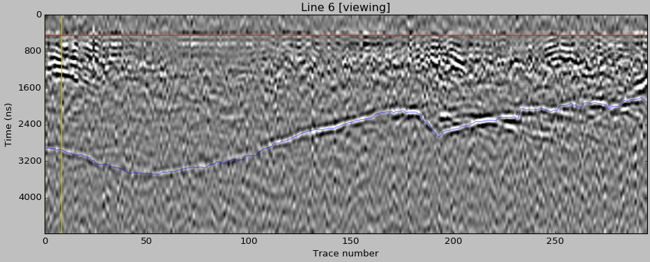
This spring we also collected data using a Ground Penetrating Radar (GPR) which transmits high-frequency radio waves into the ice. When the radio waves encounter a buried object or a boundary between materials, then it is reflected back to the surface where a receiving antenna records the signal. In our case, the bedrock surface below the ice is the surface/boundary we are looking for. Once we pick out the bedrock surface from the data, then the signal and travel time are used to then determine the ice thickness (Figure 8). Ice thickness is important for determining how long a glacier will survive as well as putting current rates of ice loss in perspective. We still have a lot of data to collect and process, but it seems that smaller glaciers like the Nordic and Zillmer (~5 km²) are 50-90 m thick in general, larger glaciers like the Conrad (16 km²) average 100-200 m thick.

Figure 8. Ground Penetrating Radar data from the Conrad Glacier. The blue line marks the bedrock surface and the red line marks the airwave, which defines the glacier surface. Between the lines is glacier ice. The longer the signal travel time, the deeper the ice. For this line, the deepest point is 220 m ice depth, and the shallowest 115 m.

Field Season Stats:

Snow Depth Measurements: 161 discrete locations, 600+ individual measurements
Snow Pits and Cores (Density): 15
- The combination of snow depth and density allow for calculation of SWE
Ground Penetrating Radar (GPR) Distance (Ice thickness, Figure 3): Roughly 75 km
- GPR data allows for the calculation of ice thickness and ice volume
Distance Skied: 200+ km
Field Team Members: 8; UNBC, CBT, UBC, ACMG.
Glaciers with both field and LiDAR data: 4/4
GPS Surveys (to corroborate field/LiDAR data comparison): 4
Days on a Glacier: 18

Season Summary: Our data indicate that winter mass balance featured a north-south trend, with the Kokanee Glacier in the south equaling last year’s mass balance, the central region was 85% of 2015 (Conrad and Nordic), and the Zillmer in the north was around 80%. The 4-6 week head start on melt season led to higher snow density in 2016 than observed in 2015. This summer melt season will determine whether the record/near record negative mass balance seen across the region in 2015 will be rivaled or exceeded in 2016. The hot, early spring has primed the region to again break records.

Clephane Bay Ice Cap, Baffin Island Being Erased from Map

On May 20, 2016May 2, 2024 By mspeltoIn Canada glacier retreat, climate change glacier retreat

Comparison of 1995 and 2014 Landsat images of ice caps A, B, C, D and E. Pink arrows indicate where A, B and E separated. C and D have disappeared. F is an outlet glacier with a retreating terminus.

The southern part of the Cumberland Peninsula on Baffin Island features many small ice caps. Here we examine the disappearance of two and the separation of two others from 1995 to 2014. Way (2015) noted that on the next peninsula to the west, Terra Nivea and G rinnell Ice Cap had lost 20% of their area in the last three decades. The retreat and disappearance of ice caps in the area have led to a INSTAAR project at UColorado-Boulder examining vegetation that had been buried and is now being exposed. Gardner et al 2011 and Sharp et al (2011) both note that the first decade of the 21st century had the warmest temperatures of the last 50 years, the period of record. They identified that the mass loss had doubled in the last decade versus the previous four for Baffin Island. This is causing ice caps like Dexterity and those around Clephane Bay to melt away

In 1995 ice caps A-E are each a single coherent ice cap, there are narrow points of connection between sections on A, B and E. Ice Caps C and D are simple ice caps between 500 and 800 m across on their widest axis. The terminus of the outlet glacier at F is an expanded lobe. Only Ice Cap A has a significant area above 800 m. The rate of loss from 1995 to 2002 is not as rapid as after, C and D still exist, A,B and E are still connected as a contiguous ice mass. In 2013 ice cap C and D are gone. The snowline is generally above A, B and E with only a small stripe of retained snow on each. Ice cap A, B and E have each separated into multiple parts. In 2014 there is no retained snow on the ice caps, pink arrows indicate the location of separation for ice caps A,B and E. In 2014 the terminus lobe at Point F has lost half of its area, retreat in distance will not accelerate. The lack of retained accumulation most years indicates no accumulation zone and the ice caps cannot survive without that. The only clear image in 2015 indicates a snowcover in August, but this appears to be from a summer snow event.