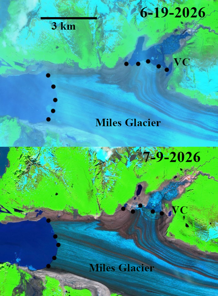
Miles Glacier and Van Cleve glacier lake (VC) near its maximum size on June 19th and after drainage on July 9th in Sentinel images. Glacier margin black dots.
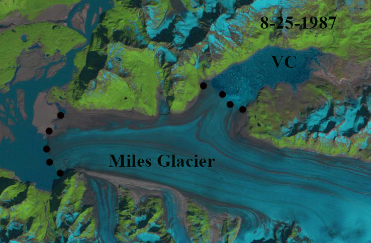
Miles Glacier terminates in an embayment on the east side of the Copper River, Alaska. A secondary terminus on the north side of the main glacier has long impounded a glacial lake that periodically drains. As miles has retreated over the last 40 years the maximum size of the glacial dammed lake has diminished, prior to its drainage. In 1987 the glacier extended onto an outwash plain directly adjacent to the Copper River, the lake reached a maximum size of 12 km2 . From 2016 to 2019 the lake drained each summer reaching a maximum average size of 5.5 km2 (Rick et al 2023). This was noted as a shrinking ice dammed lake by Field et al (2021).
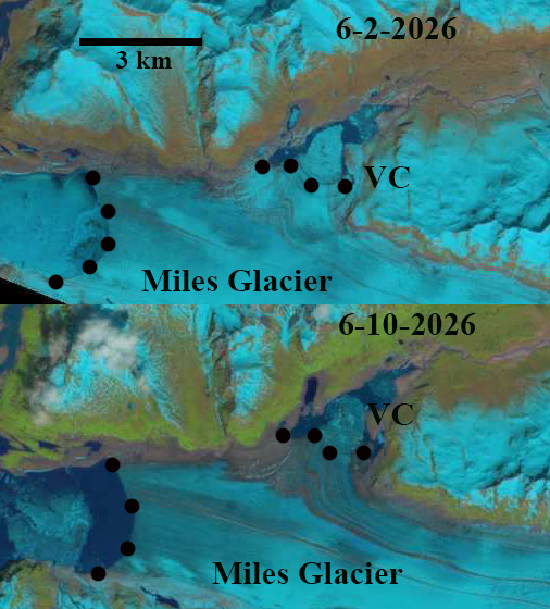
Miles Glacier and Van Cleve glacial lake filling in June 2026 in Landsat images.Glacier margin black dots.
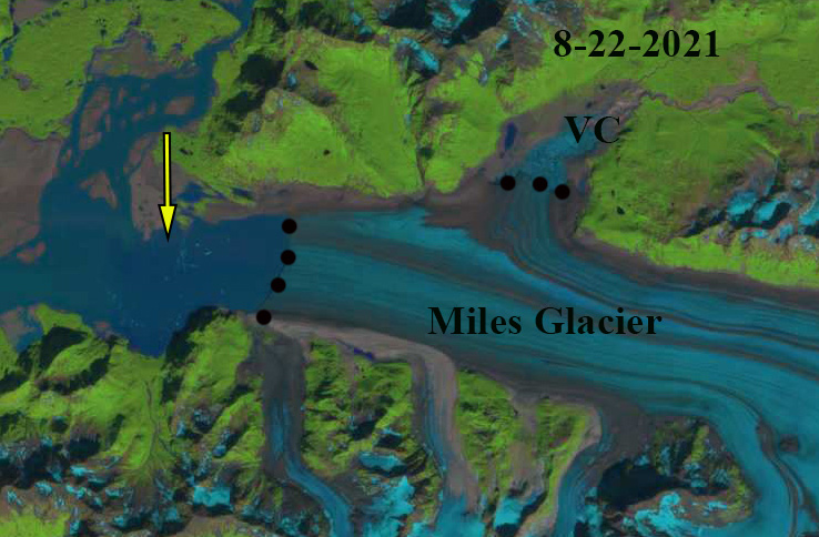
By 2021 the glacier had retreated 3.5 km since 1987. From 2021-2026 the lake reaches a maximum size of 3.5 to 4.0 km2 before draining. On June 2, 2026 the lake still has some winter lake ice and is filling. By June 10th the lake had reached 3 km2 and by June 19th it had reached 4 km2. The lake had began draining before June 25th. By July 9th it was fully drained. The Miles Glacier terminus has retreated 4.5 km since 1987. This ongoing retreat will continue to diminish the size of the lake. Ths lake does not have the complex drainage system or changing drainage location that Berg Lake has with retreat of Stellar Glacier..
Miles Glacier and Van Cleve glacial lake in 1987 Landsat image. Black dots indicate glacier margin. Miles Glacier and Van Cleve glacial lake in 2021 Landsat image. Black dots indicate glacier margin and yellow arrow indicates 1987 margin.
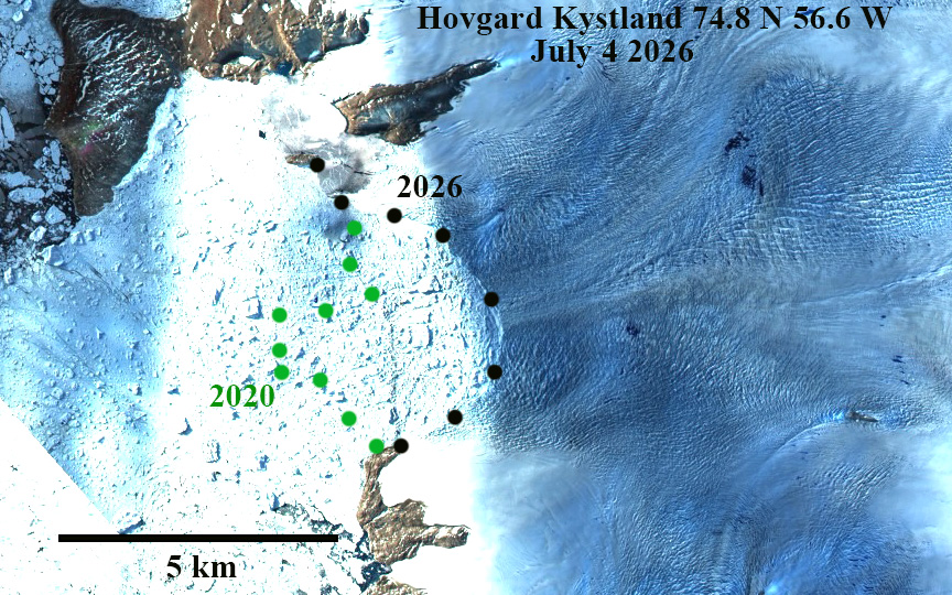
Hovgard Kystland Glacier in Sentinel image from July 4, 2026 with margin indicated by black dots. The 2020 margin seen below is indicated by green dots.
Hovgard Kystland Glacier is an outlet glacier in West Greenland between Alison and Hayes Glacier. Alison Glacier had the highest retreat rate from 1976-2021 losing 14.3 km in length and 59.4 km2 in terminus area (Black and Joughin, 2026). Hayes Glacier lost 2.7 km in length and 10.8 km2 in area (Black and Joughin, 2026).. They indicate that Hovgard Kystland Glacier retreated 5.4 km and lost 21.3 km2 during this interval.
Here we examine the acceleration of retreat from 2020 to 2026. In 2020 the central tongue of the glacier extended west beyond the main front. This central tongue collapsed by July 2024 leaving a generally north/south calving front, the glacier had lost 5.7 km2 of terminus area. From July 2024 to July 2026 an embayment formed generating a concave calving front. The glacier terminus lost another 4.8 km of area. Retreat of the calving front was 2.5 km during the 2021-2026 period. The glacier has lost an area that is 50% of the area lost from 1976-2021, in the last five years. The embayment is poised to further expand, though this summer an extensive packed melange is currently in place which typically limits calving (Meng et al. 2025).
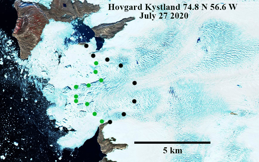
Hovgard Kystland Glacier in Sentinel image from July 27, 2020. The 2020 margin seen below is indicated by green dots and the 2026 margin with black dots.Hovgard Kystland Glacier in July 4, 2024 Sentinel image. The calving front indicated by red dots for 2024 and black dots for 2026.
Global alpine mass balance in 2024 as reported to the World Glacier Monitoring Service. Solid line is the cumulative balance, bars are the annual balance.
Each of the last 15 years I have summarized the annual mass balance of alpine glaciers globally for the Bulletin American Meterological Society-State of the Climate report,. Below is the 2024 section on alpine glaciers with a few added figures.
ALPINE GLACIERS
M. Pelto
In 2024, all 58 global reference glaciers reported a negative annual mass balance. This is only the second year in the 1970–2024 period with all negative annual balances, following 2023. The global average annual mass balance based on equal weighting of 19 regions is −1.30 m water equivalent (w.e.), the most negative value in the record
The 2024 dataset of submitted glaciological observations includes 142 glaciers from six continents and 27 nations, with 140 reporting a negative balance and 2 a positive balance. In 2024, the mean annual mass balance of the 58 global reference glaciers was −1.44 m w.e. and −1.36 m w.e. for all 142 reporting glaciers. This is a similar result to 2023, which saw a mean reference glacier balance of −1.62 m w.e. and −1.35 m w.e. for all 116 reporting glaciers.
The 2024 regionalized global average of −1.30 m w.e. exceeds the previous most negative year in 2023, which saw a regional-ized global average of −1.25 m w.e. This makes 2024 the 37th consecutive year with a global alpine mass balance loss and the 15th con-secutive year with a regionalized global mass balance below −0.5 m w.e. The acceleration of mass balance loss indicates that alpine glaciers are not approaching equilibrium. The acceleration of mass balance loss is apparent regardless of datasets used to determine it, including glaciological, geodetic, altimetry, and gravimetric observations (The GlaMBIE Team 2025). The intercomparison assessment identified that global glaciers annually lost 273+26 gigatons (Gt) in mass from 2000 to 2023, with loss having been 36% greater in the second half than in the first half of this period (The GlaMBIE Team 2025).
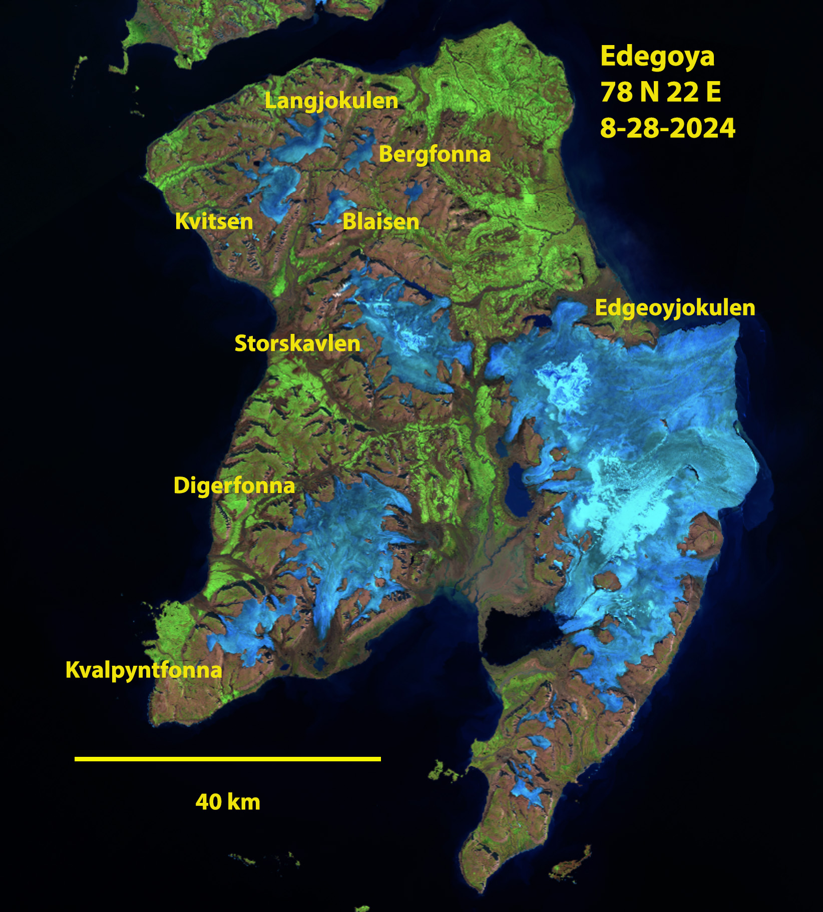
In the European Alps, all 49 glaciers reported negative mass balances, with 45 losing over 1 m w.e. All 10 Icelandic glaciers had negative balances. In Svalbard, all seven had negative balances exceeding an exceptional loss of 1.25 m w.e. This was the result of near complete snow cover loss across most glaciers (Fig. 2.20) following record temperatures in August (see section 7f5 for details). Twelve of the 13 glaciers from Norway and Sweden had mass losses of more than 1.0 m w.e.
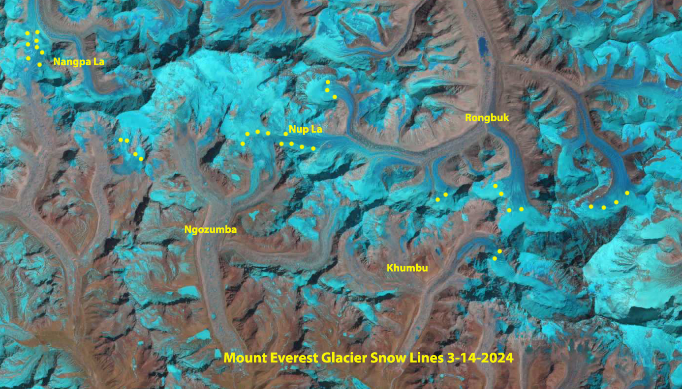
High snow line persisted through the winter on Mount Everest glaciers.
Across High Mountain Asia, 20 of 21 glaciers, reporting from seven nations, had negative balances. The highest average losses were in the Himalayas of Nepal and the lowest in the Pamir Range of Tajikistan.
In the Andes Mountains of South America, all 14 glaciers, reporting from five nations, had negative balances. Conejeras Glacier (Colombia), following a 5.04 m w.e. loss in 2023, was declared extinct in 2024. The daily hydrograph below this glacier changed from a predominanceof days with a purely melt-driven hydrograph from 2006 to 2016 to an increase in the frequency of days with flows less influenced by melt after 2016 (Morán-Tejeda et al. 2018).
All 16 glaciers in North America had negative balances. All four glaciers in Arctic Canada had mass balance losses under 1 m w.e. In western Canada and Washington and Montana (United States), all 16 glaciers reporting had losses exceeding 1 m w.e. The Ice Worm Glacier (Washington) was listed as extinct in 2023 after 40 years of continuous observations (Pelto 2024). In 2024, loss from the relict ice (ice that is no longer moving or part of a glacier) was 2.4 m and melt runoff below the glacier had decreased similar to Conejeras Glacier (Pelto and Pelto 2025). In Alaska, all three glaciers had mass balance losses. Davies et al. (2024) examined the Juneau Icefield, the most observed icefield in Alaska in terms of mass balance, and found an acceleration of mass loss with a doubling after 2010 compared to 1979–2010.
Easton Glacier, Washington extensive retreat since 1990, with last five years being the most rapid. Terminus and mass balance surveyed annually and reported to WGMS.
Alpine annual mass balance glaciological observations are reported to the World Glacier Monitoring Service (WGMS) by national representatives with a 1 December annual submission deadline. WGMS reference glaciers have at least 30 continuous years of mass balance observa-tion. Benchmark glaciers have at least a 10-year mass balance record and are in regions that lack sufficient reference glaciers. The combination of benchmark and reference glaciers is used to generate regional averages (WGMS 2023). Global values are calculated using a single averaged value for each of 19 mountain regions, limiting bias from observed regions (WGMS 2023). As this dataset expands, the annual values are reanalyzed and updated.
The lack of snow pack at the end of summer is evident across Edgeoya in Svalbard, blow a closeup of Digerfonna further illustrates with lettered points indicating new bedrock areas that are expanding amidst the ice cap.
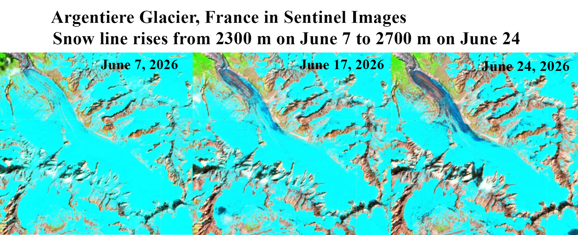
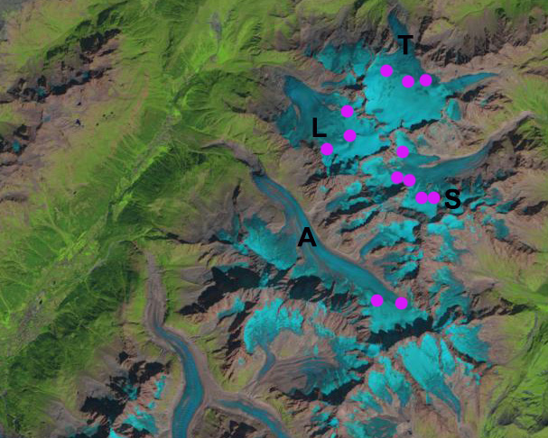
On June 1, 2026 the snowline is near the terminus of Argentiere Glacier at 2300 m, by June 24, 2026 the snowline has rise upglacier 3.3 km to 2700 m.
The French Alps have expereienced a significant June heat wave that has driven a rapid rise in glacier snow lines. Rabatel et al (2013) examined the equilibrium line altitude (ELA) of glaciers in the region from 1984-2010. The ELA is the snowline at the end of the summer melt season. Rabatel et al (2013) found the average snow line of 3000 m on Trient Glacier, 2900 m on Tour Glacier, and 2800 m on Argentiere Glacier.
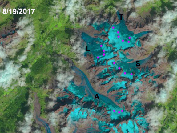
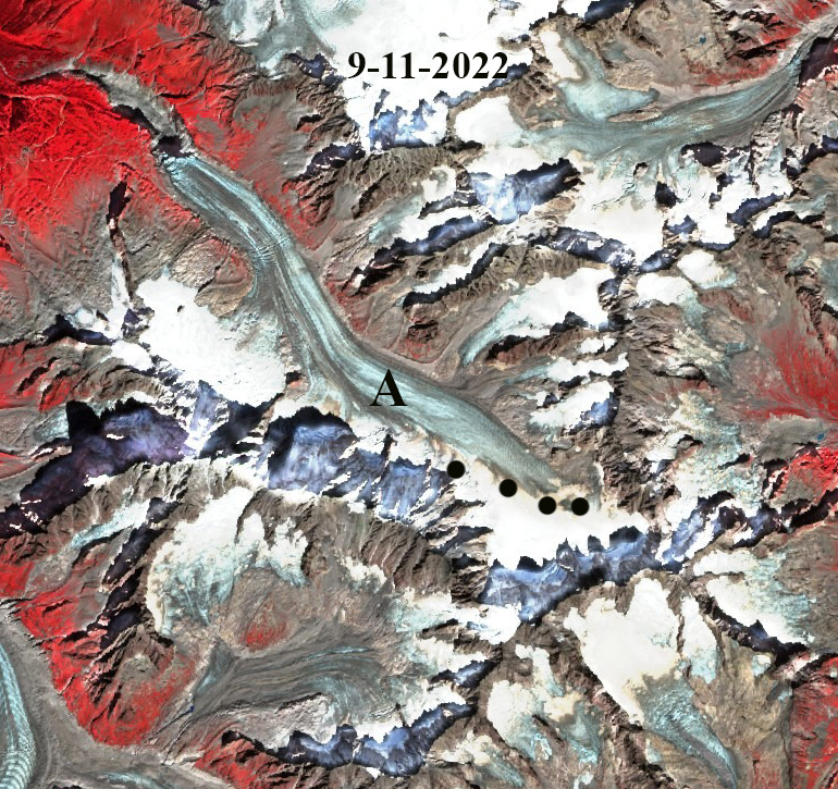
On June 1st and 7th 2026 the snow line on Argentiere Glacier was near the terminus at 2300 m, by June 24th the snow line risen to 2700 m. This is 100 m shy of the average end of summer snow line, with 25% of the glacier losing its snowcover in this period. In 2015 and 2017 the snowline reached a record height of 2950 m in late August. This snow line rose to 3000 m again in August of 2022 and to 2900 m in August 2023. The snow lines from these years are in images below
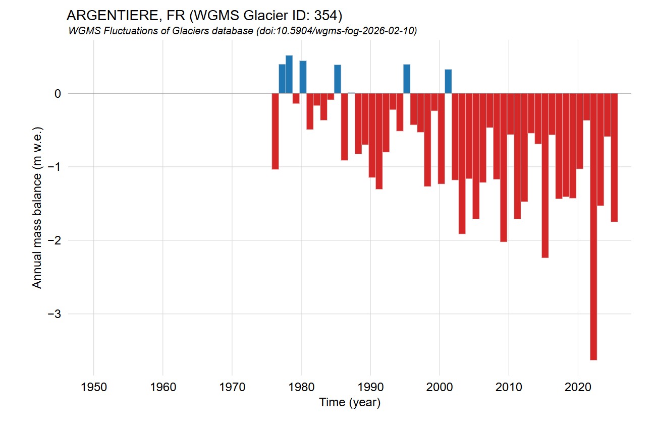
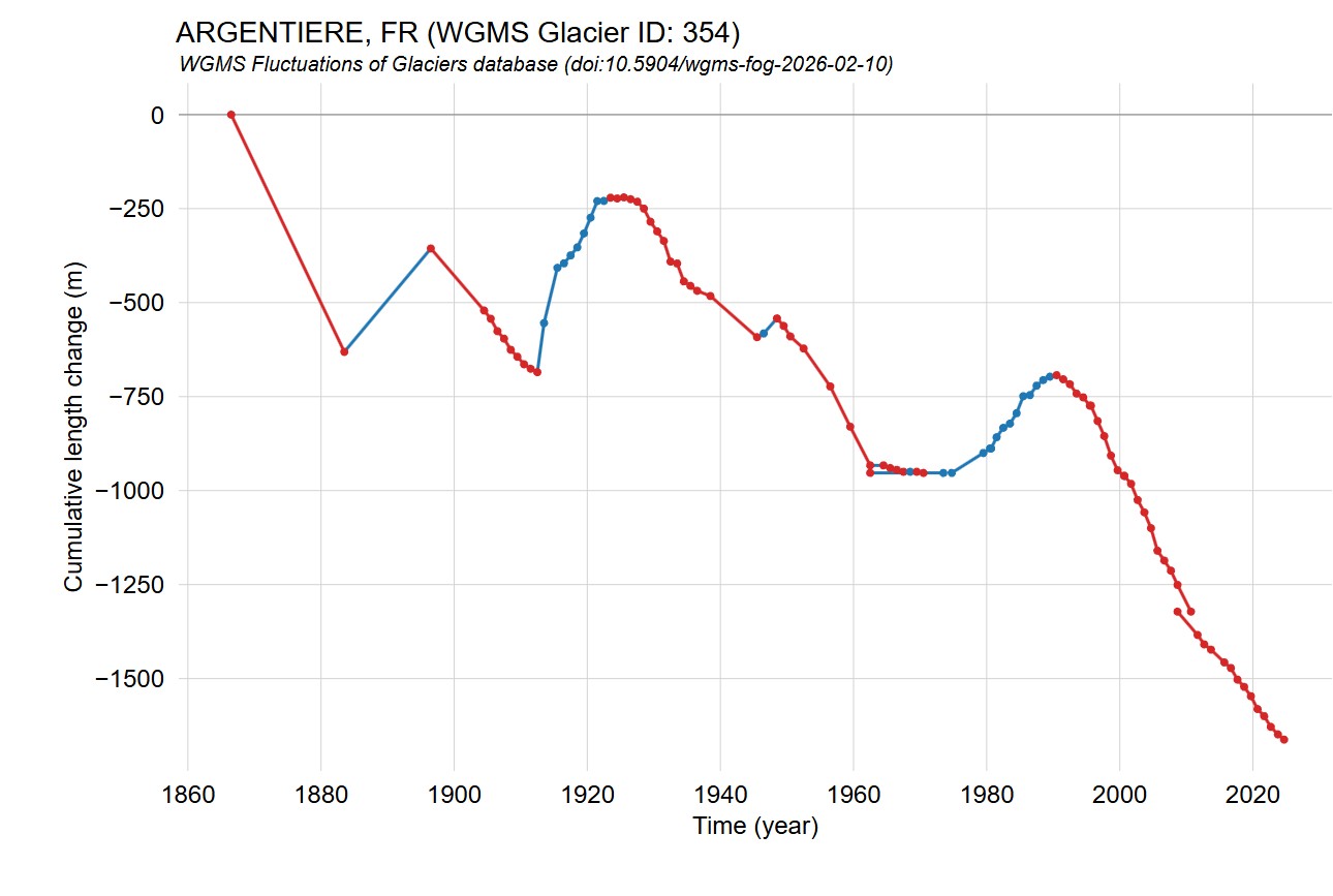
The high snow lines result in a limited accumulation zone and an expanded ablation area leading to mass balance losses and terminus retreat. Argentiere Glacier is a World Glacier Monitoring Service reference glacier, with the data indicated in the images below. The glacier advanced from the early 1960s to early 1990s and since driven by negative mass balances in all but one year this century has retreated ~ 1 km. The mass balance loss has exceeded 1 m in most years this century and will again this year.
Annual mass balance reported to WGMS for Argentiere Glacier.Terminus change reported to WGMS for Argentiere Glacier.Argentiere Glacier snow line at end of 2015 melt season at 2950 m in Landsat image.Argentiere Glacier snow line at end of 2017 melt season at 2950 m in Landsat image.Argentiere Glacier snow line at end of 2022 melt season at 3000 m in Sentinel image.Argentiere Glacier snow line at end of 2023 melt season at 2900 m in Sentinel image.
Hofsjokull East is snow free on 8-17-2025 in this false color Sentinel image. This leads to ice melt, thinning and bedrock expansion at Point A-D.
Hofsjokull East, Iceland is a small ice cap east of Vatnajokull with a summit elevation of 1100 m. In the last decade the snow line has often been above the ice cap. The ice cap had an area or 4.97 km2 in 2003 declining to 2.51 km2 in 2023 (Iceland Glacier Viewer). In 2024 all 10 glaciers in Iceland had significant mass loss (Pelto, 2025).
In August 2020 the ice cap has lost nearly all of its snow cover, this occurred again in 2023 and 2024. The result in 2025 when the ice cap again lost all its snowcover, is significant glacier surface melt and thinning. This leads to expansion of bedrock. At Point A there has been rapid expansion of the bedrock knob. At Point B and C new bedrock has been exposed and rapidly expanded. At Point D a bedrock rib at the edge of the ice cap has spread into the ice cap.
The lack of snow cover indicates the ice cap no longer has an accumulation zone and cannot survive. In 2025 the ice cap area is 2.10 km2 . Ice cap area has declined by ~60 % in the last 22 years. The story here is similar to that at the larger Prándarjökull 10 km to the northeast. The summer of 2025 in Iceland was exceptional beginning with a May heatwave, followed by a July heatwave. The May heat wave led to high snow lines as summer began on Vatnajokull.
Hofsjokull East is nearly snow free on 8-14-2020 in this false color Sentinel image. Contrast the area of bedrock at Point A-Dto the 2023 and 2025 images.
Hofsjokull East is nearly snow free on 9-3-2023 in this false color Sentinel image. Point B and C now have evident bedrock areas.
The southwest side of Kokanee Glacier from the ridge with Cond Peak at the Right and Sawtooth Ridge at center.
By Ben Pelto, PhD, UBC Mitacs Elevate Postdoctoral Research Fellow
Since 2013 I have been working on the Kokanee Glacier. Located just outside of Nelson in southeastern British Columbia (BC), the Kokanee Glacier is due north of the Washington-Idaho border. This work began as part of a five-year study of the cryosphere in the Canadian portion of the Columbia River. This project was carried out by the Canadian Columbia River Snow and Glacier Research Network — spearheaded by the Columbia Basin Trust. The glacier research, which included the Kokanee Glacier, was led by my former PhD supervisor at the University of Northern British Columbia Dr. Brian Menounos and myself. At the culmination of the project, we published a technical report, and a plain language summary of that report. When the five-year project officially ended in 2018, I learned of a BC Parks program called Living Labs, which offers funding for climate change research in BC Parks, particularly research which documents change and guides protected area management. With Living Labs funding in 2019-2021, I have kept the annual mass balance trips going — now a continuous nine-year record — and a winter mass balance trip in 2021. In conjunction with this, Brian Menounos has secured continued funding (continued from our 5-year project) from BC Hydro for LiDAR surveys of the glacier every spring and fall. These surveys are carried out by the Airborne Coastal Observatory team from the Hakai Institute.
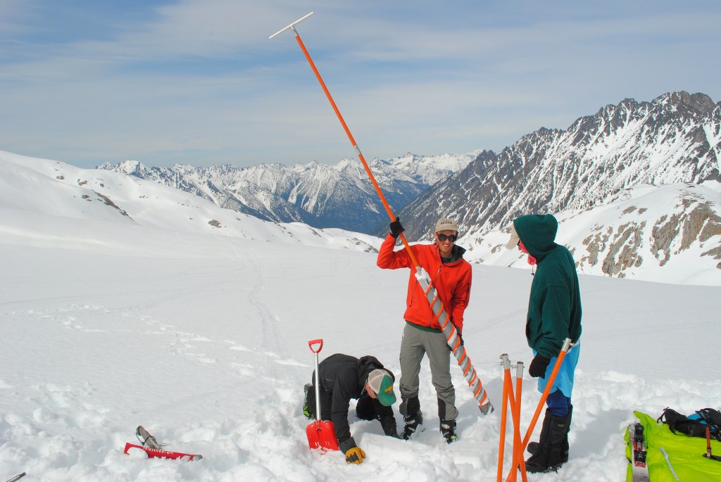
During the 2021 spring trip, we found that the Kokanee Glacier had an average snow depth of 4.4 meters. Using snow density measurements collected with a snow-corer, we found that the winter balance for 2021 was 1.91 meters water equivalent (m w.e.). This value was lower than the 2013-2020 average of 2.18 m w.e. (Pelto et al. 2019).
Ali Schroeder probing snow depth on the Kokanee Glacier while Joel McBurney and Drew Copeland look on.
Ben Pelto with the snow corer with Tom Hammond and Micah May on Kokanee Glacier. Photo: Jill Pelto
With a below average winter balance, 2021 would need to feature a cool summer. Instead, multiple heat waves occured, with temperature records being broken across the province. Wildfires burned all over BC and the neighboring US states of Washington and Idaho, swamping the region in smoke for weeks on end. Rather than mitigate for a slightly-below-normal snowpack on the Kokanee, summer 2021 took a blow-torch to glaciers across the region.
We hiked into the Kokanee Glacier on September 12, stopping under a boulder to wait out proximal booms of thunder and flashes in the clouds. We got pelted with bursts of both hail and graupel, and soaked in the rain, before gingerly working our way up boulder field and talus that is climbers route up the Keyhole to the Kokanee Glacier. Like the satellite imagery had shown, there was no snow in sight on the glacier — bare ice only. Instead of my usual camp on the snow, we chose a climbers bivy site to set our tent.
Camp in the Keyhole — a total lack of snow forced us to skip camping on-glacier.
The Keyhole route, a challenging scramble with 43 lb packs.
Stepping out onto the glacier, we immediately ran into difficult terrain, crevasse bridges of snow or firn had collapsed, leaving bedroom-width crevasses gaping open, necessitating an exercise in maze navigation. Our first stop was a stake at 2600 m which typically retains snow (50 to 100 cms), but this year had lost 1.6 meters. In fact, two stakes drilled at the site in 2015 and subsequently buried by snow had melted out, demonstrating that all snow/firn from the intervening years had been lost. This observation clued me in to the magnitude of melt to expect this year.
The first stake visited, showing 1.6 m of melt
Exposed layers of firn in a crevasse by the stake, showing 1.5 m-thick annual layers — now being eaten away by melt.
Travel on the glacier was more challenging in spots, but overall faster, as the total lack of snow meant that most crevasse bridges were gone, requiring less probing of crevasse bridges and roped-travel. Later, using a satellite image from the dates of our visit, I mapped the retained snow cover, limited to two tiny patches high on the glacier’s east side. The accumulation area ratio (AAR), or the ratio of snow cover to bare ice/firn was <0.01, meaning that under 1% of the glacier was covered in snow.
The upper reaches of Kokanee Glacier to Cond Peak (2800 m) with no retained snow in 2021. Bare ice is exposed on the lower half of the image, and firn, or multi-year snow above
The brown surface is multi-year firn, exposed by the loss of snow. In a typical year, the snow line would be visible here. The white surface below the brown is bare glacier ice.
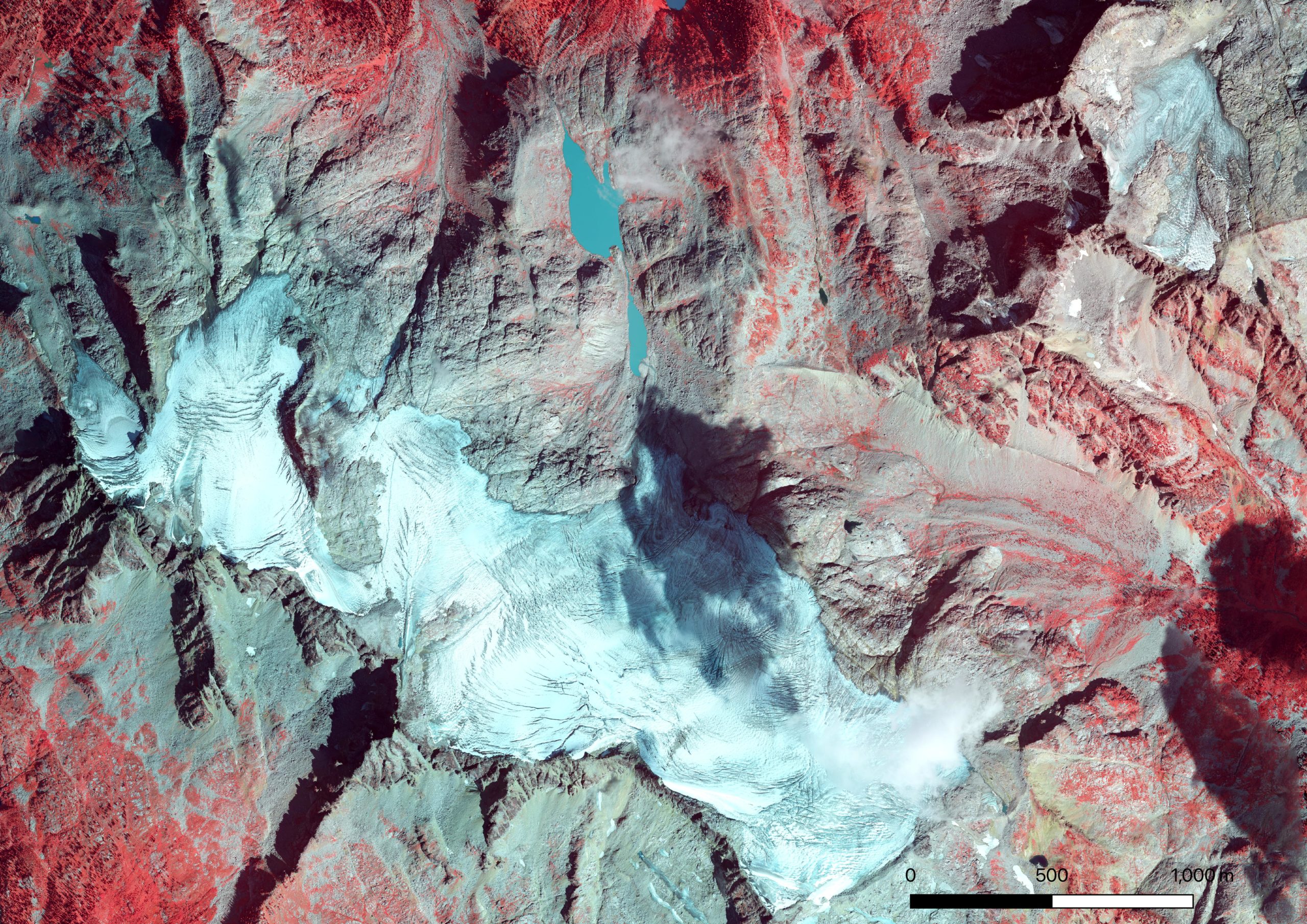
Near infrared-Red-Green 30 cm resolution ortho image of Kokanee Glacier from the Hakai Geospatial/ACO team on Sept. 2, 2021. Note how badly crevassed the glacier is, most crevasses are exposed with no retained snow. The white color and mottled appearance over the upper glacier is a skiff of overnight snow just a few centimeters thick that melted off the next day. Also note bare ice patches exposed under formerly perennial snow patches that have shrunk in recent years and now are disappearing.
Visiting the toe of the glacier, our lowest stake indicated just under 5 m of ice melt, double that of 2020. In May, this location had 3 m of snow; the combined melt of snow and ice (loss of winter snow and glacier ice) is termed the summer mass balance, and at this site was -6.2 m w.e., far higher than the usual -4 m w.e. I also noticed that much of the thin ice along the margin of the toe was gone, and a little rock nunatak (rock island) that appeared in 2015 (images below) became a bite out of the glacier rather than a island. We estimated that the toe experienced 60 m of retreat. Over the past 5 years, the Kokanee has lost an average of 16 m in length annually. Expecting to see above average thinning and retreat, I was still startled to see how diminished and thin the toe looked.
2015: a small hole forms in the glacier margin above the toe, Jesse Milner in the foreground
2021: the hole is now a bite out of the glacier with two prominent rock knobs
A week prior to my field visit, the Hakai Institute ACO team flew a LiDAR survey of the Kokanee Glacier as part of their work with Brian Menounos at UNBC. Comparing this year’s glacier surface with that from last year’s survey, Brian found a whopping 2.55 m of thinning. After mapping the glacier facies (ice/firn/snow) to represent on the density of the observed thinning, this equates to a glacier mass balance of -2.16 m w.e., higher than the previous record loss of -1.20 m w.e. in 2015.
LiDAR-derived height change 2020 to 2021 from 1 m resolution DEMs from Brian Menounos and the Hakai Institue ACO team. The black line is the 2021 glacier outline, note the bite out of the glacier above the toe to the NE corner of the glacier. Small red patches off-ice are seasonal snow patches losing mass. Points represent mass balance observation locations.
Kokanee Glacier terminus from 2015 to 2021. 140 meters of retreat for 23 m/yr. Data in the GIF are from Hakai Institute and Brian Menounos of UNBC ACO glacier surveys.
Back home, I crunched the numbers from our glaciological observations of mass balance (consisting of 14 ablation stakes this year) and calculated a mass balance of -1.97 m w.e. With Brian, I published a paper in 2019 (Pelto et al. 2019) comparing glaciological (field) and geodetic (LiDAR) mass balance estimates and found them to be similar — if some factors like snow and firn density were carefully considered. The small difference between estimates is likely due to timing (the LiDAR mass balance is from 8/26/2020 to 9/3/2021, while the field mass balance is 9/12/2020 to 9/13/2021), and that there was a skiff of fresh snow (likely 5-10 cms) on the glacier during the 2020 LiDAR survey.
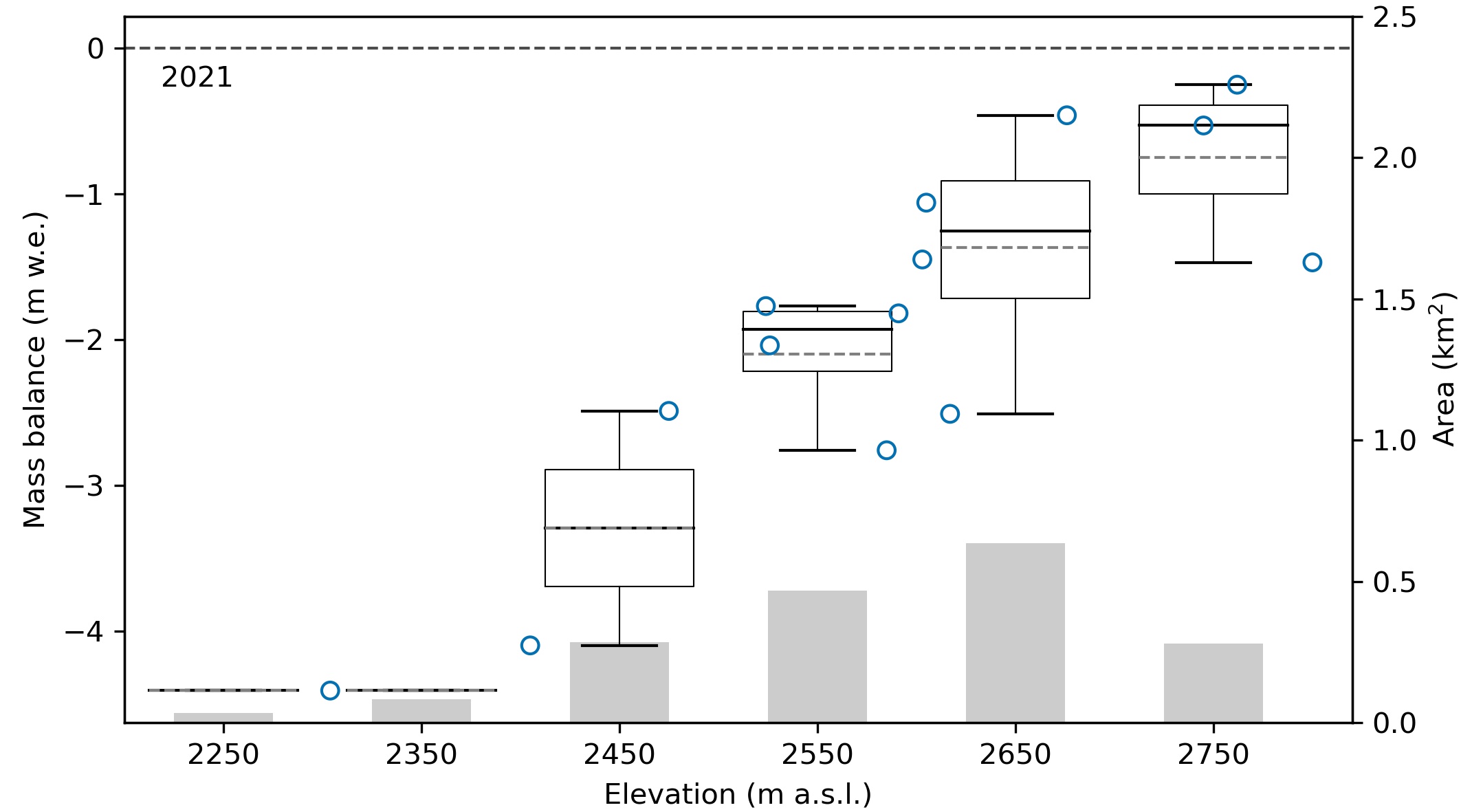
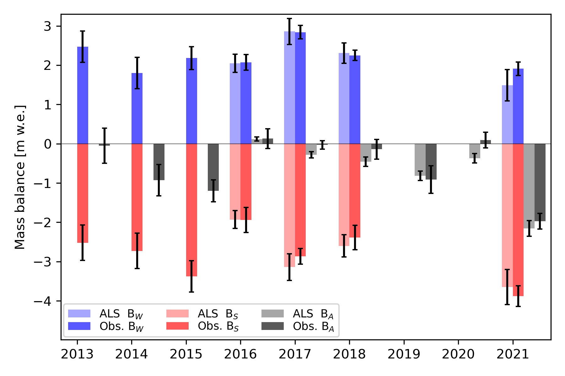
Kokanee 2021 glacier mass balance. Blue dots are observations. The boxplots show the 100 m bins used to estimate glacier-wide mass balance (median line in black, mean dashed grey line). The grey bars depict the area of the glacier for each 100 m elevation-band
Seasonal and annual mass balance for Kokanee Glacier from LiDAR and glaciological measurements for each balance year from 2013 to 2021 with 2σ uncertainties.
In 2017, I visited the Kokanee Glacier to measure it’s ice thickness using ice-penetrating radar. I found that the glacier on average was 43 m thick using my measurements to tune a glacier model. I published these results in the Journal of Glaciology (Pelto et al. 2020). In the five years since that work, the glacier has lost over 4.8 m of total thickness. That equates to a loss of over 11% of its total volume. 2021 alone wasted away 6% of the glacier’s total volume — an eye-watering number for a single year.
Cumulative mass balance for Kokanee Glacier 2013-2021 from both field and LiDAR measurments. LiDAR-derived mass balance began in 2016.
The heat of 2021 was an outlier, but years like 2021 and 2015 take a toll on the glaciers. Currently, glaciers in western North America are losing around 0.75 m of thickness per year (according to my work in the Columbia Basin (Pelto et al. 2019) and work by Brian Menounos for all of western North America (Menounos et al. 2018)). The better years for Kokanee Glacier (2016 mass balance: +0.12 m w.e.) pale in comparison. That meager surplus was lost the very next year (2017).
Herein lies the issue, positive mass balance years in recent decades are not large enough to offset even average years; hot dry summers take years off the lifespan of glaciers across western North America.
Losing 6% of it’s total volume in 2021, the best we can hope for Kokanee Glacier is a few near-neutral or positive mass balance years to cover back up the exposed firn, to keep the glacier albedo from becoming too dark and increasing the rate at which ice can melt.
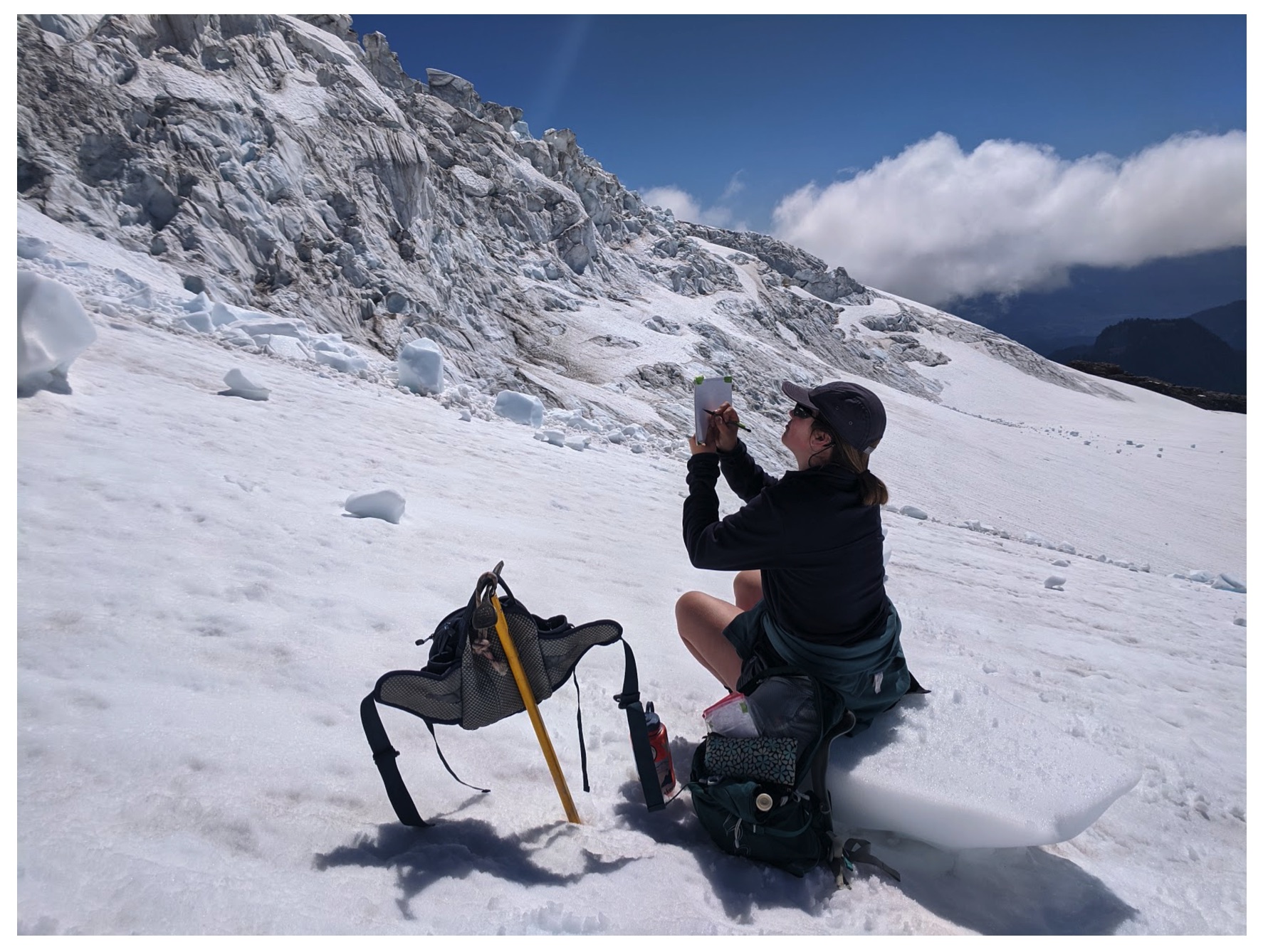
The field team at Camp discussing science communication and gazing at the Easton Glacier. Photo by Jill Pelto
By: Cal Waichler, Jill Pelto, and Mariama Dryak.
It is the evening of Aug. 9th, 2020 and six of us are camped near the terminus of Easton Glacier. The sun has dropped below the moraine ridge above camp and a chilly breeze has forced us to put on layers. We are enjoying dinner cooked on our camp stoves, discussing what we observed on the ice today. The toll of climate change on Easton Glacier, on the southern flank of Mount Baker, is impossible to escape. We are here to both measure this change and communicate what it means.
Within our team of six, four of us are trained as scientists, and all of us highly value creative science communication. This passion can manifest as art (painting, printmaking, sketching), writing, podcasting, blogging or video-making. We all appreciate that exercising creativity with others can provide us with a unique context for communicating about glaciers and climate change.
Cal creates at Columbia Glacier–sketching and taking notes to capture the power of our lunch spot that day. Photo by Mariama Dryak.Jill paints the icefall. Photo by Mariama Dryak. .
The Easton Glacier is large and stretches up to 2950 m elevation. We are here to monitor its health for the 31st consecutive year: its snow coverage, snow depth, terminus retreat, change in surface profile, and its annual mass balance (snow gain vs. snow loss). Easton Glacier is one of the forty-two World Glacier Monitoring Service reference glaciers, meaning it has 30+ consecutive year of mass balance observations, qualifying it for this select group. To learn more about this glacier over time, check out https://glaciers.nichols.edu/easton/ and a previous Easton Glacier update.
While we are at Easton Glacier to measure annual changes, we also see this landscape in the realm of both art and science. From the artistic lens we may note the same things that we do during research: the debris covering the retreating terminus, the crevasses melting down and getting shallower. But we also notice the beauty of these structures, how the crevasse patterns splay out across a knob, and the parallel lines preserved on a serac – recording five years of accumulation like rings on a tree. Observation is a theme in both art and science. We train our eyes to notice things in different ways, to pay attention to certain details. We are able to document these changes in our field notebooks, but also in sketchbooks, journals, photos, and videos.
The records of beauty stored in our sketchbooks serve as a qualitative reminder of what this landscape looks and feels like. In the process of depicting the landscape at the end of a field day, we paint our joy and exhaustion onto the page. In the moment, this act uncovers more details and allows us to reflect. Weeks later when we are off the mountain, we reopen our water-logged, dirt-streaked pages and are taken back to that place where we were. Field sketches, poems and paintings help us capture the emotion of moving through and attempting to understand sublime spaces. They are a vital link between our memories and sharing the meaning of our experience with others. They are also a deliberate recording of time and place — a kind of data in their own right.
The experience of working in this environment is memorable to us — we get to observe a plethora of crevasses, dozens of meltstreams, and strikingly beautiful colors. We can feel a range of excited, inspired, and nervous emotions throughout the day. For us, this experience is giving us the emotional context to our research: being present we can understand that “why”. That reason why the work matters not just for scientific knowledge, or the local ecosystem, but also for humanity. The science results alone can share the data that underlies that, but they might not always connect with other people in a way that elicits that comprehension. Our creative communication through writing and art can elicit that deeper, emotional understanding of why it’s important to preserve and protect these places, and why we need to understand the amount of change that will occur to the climate and ecosystem. Our collection of art shares stories about Easton Glacier in ways that connect with the science, and also go beyond it.
This summer we all felt especially fortunate to be in the North Cascades. Covid-19 has kept us all so isolated and often indoors. The chance to work on the glaciers and live at their feet for two weeks gave us back some of the breathing room we lacked in 2020 – a lucky opportunity indeed.
The American Geophysical Union Fall meeting’s Cryosphere section continues to grow as seen in the Poster hall. The poster hall is where most of the research is presented and is dominated by student work. Here are some examples of this work.
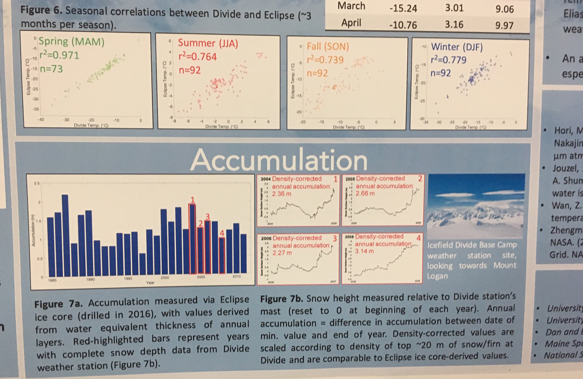
Erin McConnell, UMaine and others examined shallow ice cores from glaciers in the St. Elias Mountains of Canada’s Yukon as part of a project to reconstruct past climate variability using ice cores. The study quantified the relationships between meteorological data and ice core records in the St. Elias. The focus was on Icefield Divide, 2,900 m and Eclipse Icefield, 3,017 m. In June 2018 they extracted two ice cores (10 m and 20 m) from Divide. at Eclipse. In addition they did a 400 MHz radar transect at Divide which showed a strong reflectance at ~30 m depth, that likely indicates a firn aquifer, that develops from meltwater percolation and causes the isotope signal to deteriorate below the 2017/2018 snowpack (~6 m depth). GPR data from Eclipse Icefield shows no evidence of an aquifer, suggesting the process in the St. Elias may occur only below ~3,000 m elevation. The results pictured contrast annual accumulation at the two sites.
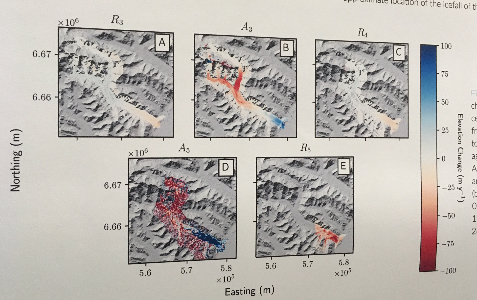
Andrew Nolan and others, from UMaine examined the surging Turner Glacier. Surge glaciers exhibit a short active phase of rapid ice velocity followed by a longer quiescent phase of slower flow. Turner Glacier is in the St. Elias Mountains, Alaska adjacent to Hubbard Glacier. Using a Landsat archive for the 1984 to 2017 period they found five previously unexamined surge events. Surge events occurred in 1985-1986, 1991-1993, 1999-2002, 2006-2008, and 2011-2013. This indicates a ~5-year surge repeat interval. They used ASTER digital elevation models from the 2006-2007 and 2011-2013 to show mass build up in the reservoir zone which initiates the surge, prior to the surge. The surge then redistributes the mass to the terminus zone. The reservoir zone surface elevation increased 50 meters preceding the 2005-2008 surge event and then subsided 100 meters and the terminus zone rose 75 meters. The image below indicates thinning in red upglacier and thickenning in blue downglacier.
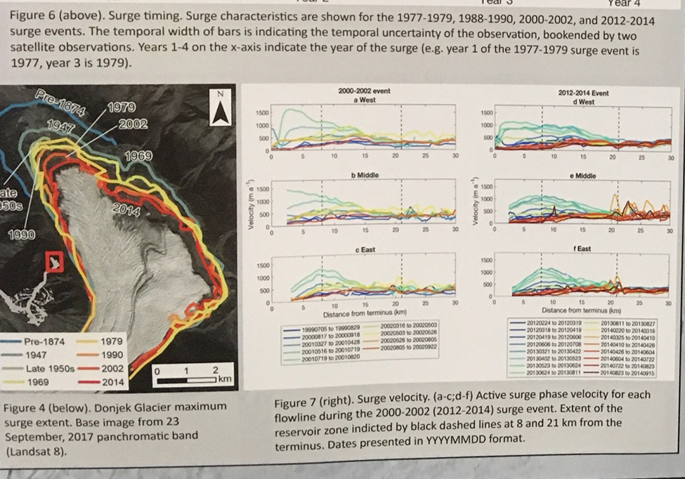
Wiiliam Kochtitzky, UMaine and others examined Donjek Glacier a surging glacier in the St. Elias range, Yukon. They examined velocity and ice elevation changes since 2000 on this 65 km long glacier to understand the beginning and end of surges. The glacier has surged eight times since 1935 with a 12 year repeat rate. The glacier has had a negative mass balance and has retreated 2.5 km since ~1874. Each successive surge of Donjek Glacier has featured a more limited advance than the previous. This akin to waves on a falling tide. To map ice motion before, during, and after the 2001 and 2013 surge events they used Landsat scenes to measure monthly ice velocity. During these events they observed maximum uplift of ~75 m in the terminus (receiving) zone and maximum subsidence of ~65 m in the reservoir zone, 8-21 km above the terminus. The most negative mass balance occurred in the lower 32 km of the glacier after the 2013 surge, with Donjek losing an average of -6.65 m year. The upper 40 km of the glacier is not involved in the surge. This glacier has important implications for larger ice masses, such as ice streams, that could have strong negative mass balances even if they surge and/or are land terminating superimposed on the surge cycle.
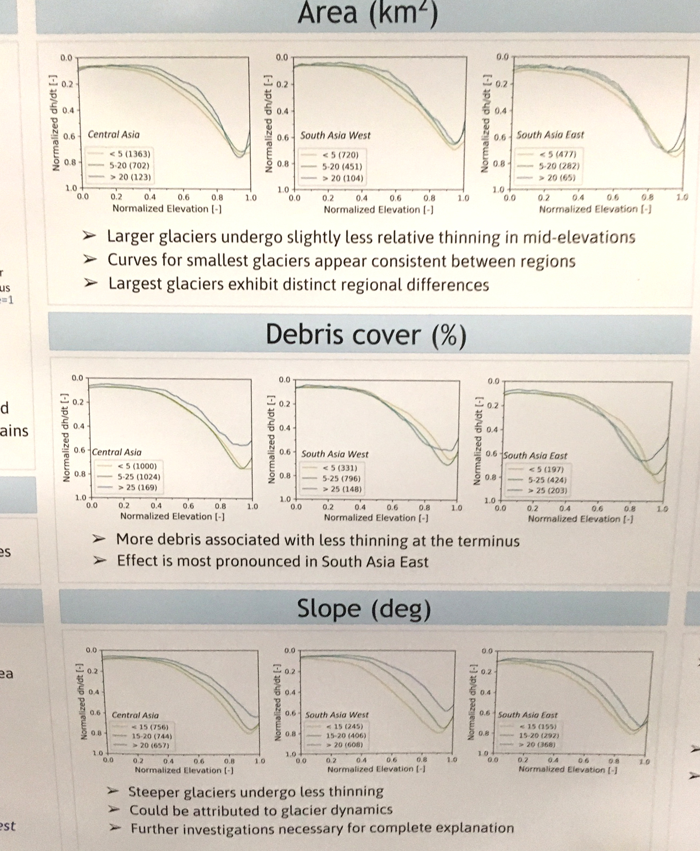
Pacifica Askitrea Takata-Glushkoff of University of Alaska Fairbanks and others examined the glacier dynamics of High Mountain Asia (HMA) glaciers. She used a glacier evolution model to account for geometry changes from surface mass-balance feedback. Previously used scaling methods are simpler than flow models, but they do not account for glacier thinning. Glaciers typically show most thinning at lower elevations and least thinning at higher elevations, with various factors influencing these relative thinning patterns. She investigated glacier thinning variability with elevation, in order to account for retreat . Using geodetic data from 170 glaciers in the High Mountain Asia region, they determined for each glacier how normalized changes in ice thickness vary with elevation. They investigated whether those normalized curves are impacted by factors such as glacier area, slope, aspect, debris cover, length, and glacier terminus elevation. Results indicate that shallow slopes and less debris cover are both associated with more relative glacier thinning toward the glacier terminus.
Andrew Hengst and others from Appalachian State University mapped pro-glacial lakes in Northwestern North America to better understand . They used a semi-automated algorithm to delineate proglacial lakes and analyze proglacial lake area change over the satellite record to investigate lake growth rates and physical controls. This approach allows robust identification and analysis of proglacial lake area change utilizing the complete Landsat satellite record . The use of an object-based processing algorithm enabled automatic location and tracking proglacial lakes over large spatial and temporal scales to increase understanding of the dynamics of these complex and changing systems, such as in the examples below that show lake area change. The algorithm had the most difficulty with lakes that had high suspended sediments and debris covered termini with a complex ending in the lake.
During the last six years From a Glaciers Perspective has published 520 Posts examining the response of glaciers to climate change. No hyperbole has been needed to use words such as disappear, fragmented, disintegrated, and collapse. Glacier by glacier from the fragmentation of glaciers to the formation of new lakes and new islands has emphasized the changing map of our world as glaciers retreat. The story details change, but the story remains the same; glaciers are poorly suited for our warming climate, and their only response is to hastily retreat to a point of equilibrium, which many will not attain, and some have already ultimately failed. The Gallery below is a mere snippet of the changes that are occurring. These are illustrations of why our paper this year led by the World Glacier Monitoring Service team was titled Historically unprecedented global glacier decline in the early 21st century. As the UN Climate Change Conference 2015 in Paris, COP21 begins, since no glaciers are invited, there story must be told in pictures, data and our words.
Data: World Glacier Monitoring Service Mass Balance Time Series for Alpine Glaciers.
Pictures
Words:
After 34 consecutive summers working on glaciers, there is occasion to speak as more than just a scientist, since glaciers do not have a voice people hear.
The Gilkey Glacier is a 32 km long outlet glacier flowing west from the Juneau Icefield. From 1948 to 1967 the Gilkey Glacier retreated 600 m and in 1961 a proglacial began to form. By 2005 Gilkey Glacier has retreated 3900 m from the 1948 terminus location. The glacier is currently terminating in this still growing lake, notice the new bergs and rifting at the glacier terminus. The retreat has been resulted from and in a thinning of in the lower reach of the glacier and the separation from Battle and Thiel Glacier. A major tributary to Gilkey Glacier, is Vaughan Lewis Glacier. At the base of the Vaughan Lewis Icefall where the Vaughan Lewis Glacier joins the larger Gilkey Glacier ogives form, as seen from above and below the icefall (Scott McGee). The ogives form annually and provide a means to assess annual velocity in this section of the glacier. Aerial photography of the ogives from the 1950’s combined with current satellite image provide the opportunity to assess ogive wavelength over a 50 year period, providing a long term velocity record for Gilkey Glacier. An ogive is a bulge-wave that forms annually due to a seasonal acceleration of the glacier through an icefall. The acceleration is enhanced in icefalls that are horizontally restricted. In most cases we do not have specific measurements of velocity through all season to ascertain the timing of the accelerated period, though typically spring would be the fastest. After formation the bulges move down glacier and a new bulge is formed the following year. The resulting train of ogives extending down glacier can be used to estimate the ice velocity by measuring the peak to peak separation between adjacent waves. Ogives can be visually identified as a series of arcuate wave crests and troughs pointing down glacier. Downglacier from this formation point the crests and troughs gradually flatten until the ogives are merely arcuate light and dark bands on the surface of the glacier. The dark bands are dense, blue and dusty ice that is compressed during summer, whereas the light bands are bubbly, white, air-filled ice that is compressed during winter.
In 1981 one of my tasks was to ski out through the top of the icefall inserting stakes in the crazily crevassed region to track summer velocity for the Juneau Icefield Research Program (JIRP). This has been completed often but not most years by JIRP. What we discovered was that velocity in 1981 had not changed from the 1960’s and 1970’s. Today we have frequent satellite imagery of the ogives to ascertain annual velocity that can be compared to the few aerial photographic records, in this case from 1056 and 1977. In several recent years Scott McGee of JIRP has specifically surveyed the distance between the first 11 ogive crest below the icefield. A comparison of the the ogives in 1956, 1977 and 2005 is possible by overlaying the images below. . The distance from the first to the 40th ogive has gone from 6.8 km in 1956 to 6.75 km in 1977 to 6.2 km in 2005. In 1956 and 1977 the first ten ogives spanned 1500 meters indicating an annual glacier velocity of 150 meters. From 2003-2007 the distance of the first ten ogives averaged 1440 m, or 144 meters per year. The change in velocity is quite small, compared to the large retreat of the glacier. One other key measure of the ogive surveying program is the surface elevation. A longitudinal profile containing 179 survey points was established at the base of the Icefall in 2001-2007. This profile begins in the trough immediately upglacier of the crest of the first wave ogive and continues downglacier nearly 1.8 kilometers to a point where the amplitude of the ogives becomes zero (Graphs and data from JIRP) During this six year time period, the surface has lowered an average of 17 meters – nearly 3 meters per year – along the longitudinal survey profile, with a maximum of 22 meters. This substantial thinning at the base of the icefall indicates reduced discharge through the icefall from the accumulation zone above. This will lead to further retreat and velocity reduction of Gilkey Glacier.
The Cordillera Blanca, Peru has 27 peaks over 6,000m, over 600 glaciers and is the highest tropical mountain range in the world. Glaciers are a key water resource from May-September in the region, Mark (2008). The glaciers in this range have been retreating extensively from 1970-2003, GLIMS identified a 22% reduction in glacier volume in the Cordillera Blanca. Vuille (2008) noted that the retreat rate has increased from 7-9 meters per year in the 1970’s to 20 meters per year since 1990. One of the glaciers that is continuing to recede is Llaca Glacier descending the west slopes of Ranralpaca. This glacier has retreated 1700 m from its Little Ice Age moraine, outlined in lime green. Llaca Laguna is impounded by this moraine. The glacier still has a significant consistent accumulation zone and can survive current climate. Stagnant pockets of debris covered ice no long connected to the glacier fill much of the valley between the laguna and the current glacier. The terminus despite ending on a steep slope lacks significant crevassing indicating a lack of vigorous flow which will lead to continued retreat of 20-30 meters per year. This glacier drains into the river which then flows into the Rio Santa in Huarez, Peru. Mark (2008)note the importance of glaciers to the Cordillera Blanca watersheds in the Huarez region receive 35% of their runoff from glaciers, and the upper Rio Santa likely receives 40%.