Desolation Valley, Alaska, Conversion from Glacier to Lake


desolation-compare

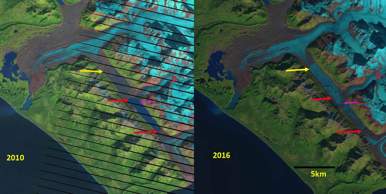
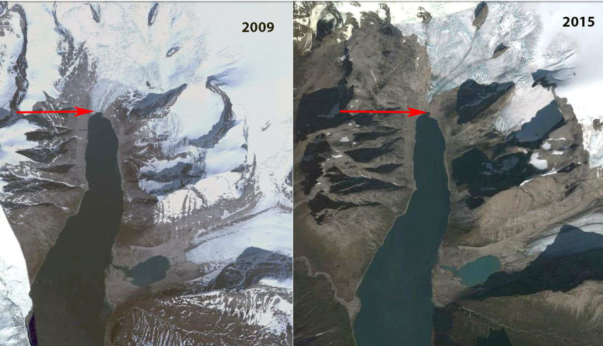
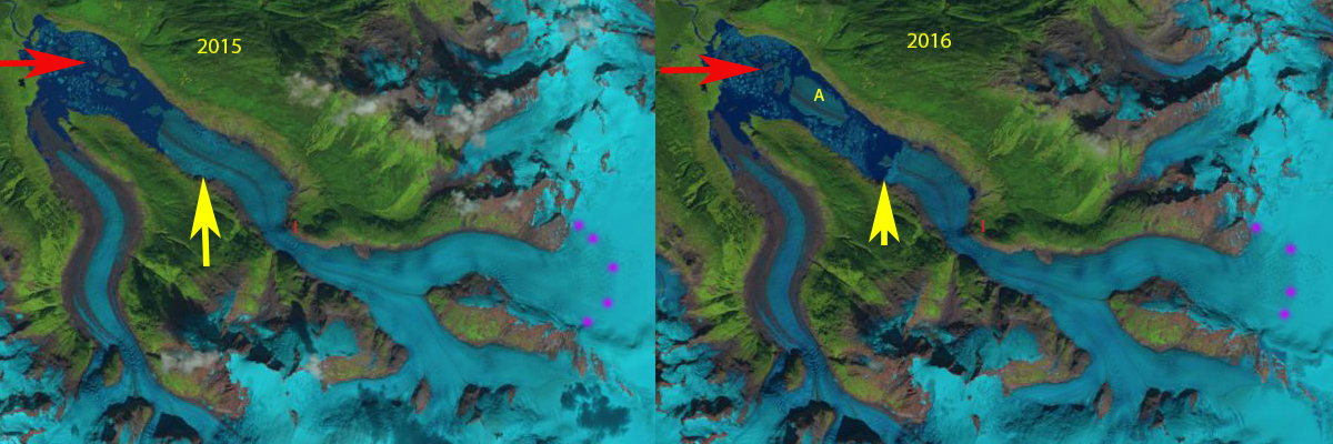
Retreat of Desolation-Fairweather Glacier from 2010-2016 in Landsat images.  The red arrow indicates 2010 terminus positions, yellow arrow the 2016 terminus. Pink arrow a delta exposed by lake level lowering. D=Desolation Glacier.

Desolation Glacier flows west from the Fairweather Range into Desolation Valley where in 1986 it joined with the Fairweather Glacier flowing from the north and the Lituya Glacier flowing from the south to fill the valley with glacier ice.  This is no longer the case, the valley once known for its long relatively flat area of largely debris covered ice, is mostly a lake now.  The valley has developed along the Fairweather Fault. Molnia (2007) noted that the tidewater termini of Lituya Glacier advanced ∼ 1 km since 1920 and continued to advance up to 2000 as it built an outwash plain reducing calving. Larsen et al (2015) noted thinning rates of 3 m per year for the Desolation Valley from Desolation Glacier north to Fairweather Glacier in the last decade (1994-2013).  Alifu et al (2016) identified that Desolation Glacier and Fairweather Glacier have lost 2.6% and 2.2% of their glacier area, respectively from 2000-2012. Only minor surface area changes were seen in Lituya Glacier during this period. They also noted that the mean snow line altitude of Fairweather, Lituya and Desolation increased by 120–290 m. Since 2012 extensive ice loss of the Desolation-Fairweather complex has occurred.  This is similar to the large rise in the transient snowline/equilibrium line noted by Pelto et al (2013) on nearby Brady Glacier.

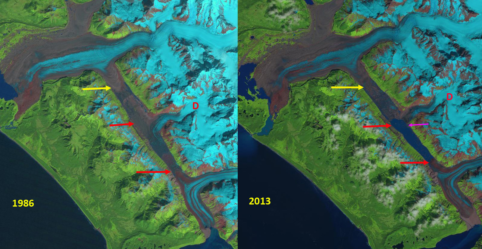
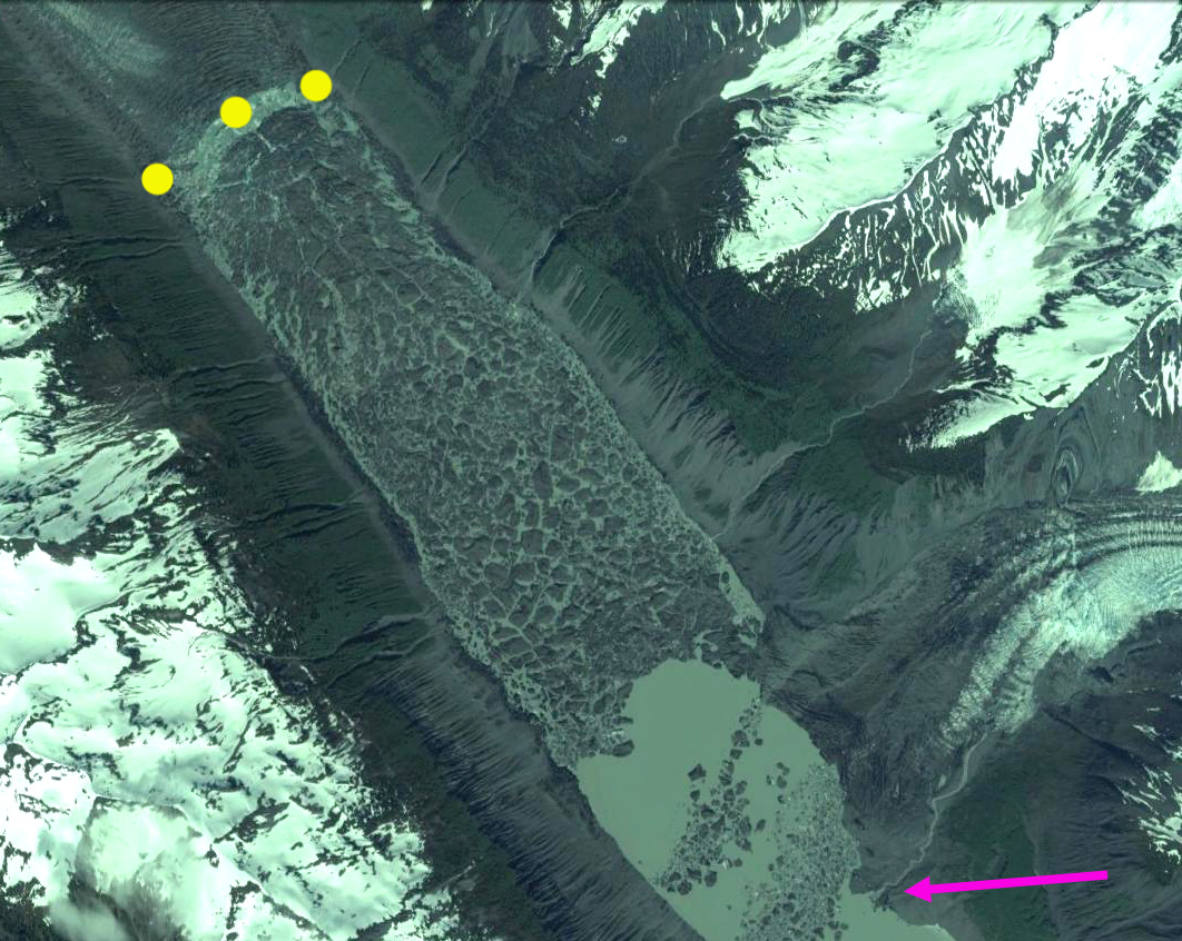
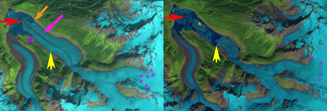
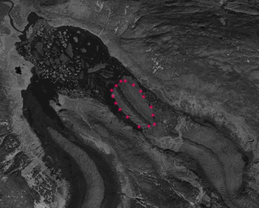
In 1986 The Desolation Valley was filled with glacier ice from Fairweather Glacier to Liutya Bay.  By 2010 the southern half of the valley from Lituya Glacier to the outlet of Desolation Glacier into the valley had opened up and the terminus of Desolation Glacier and Lituya Glacier were at the red arrows, this represented a 5.3 km section of glacier lost. In 2013 the northern half of the valley filled by the Desloation-Fairweather Glacier was breaking up but still ice filled.  The Google Earth image from 2014 illustrates how broken up.  By 2016 the collapse was total and the new terminus is at the yellow arrow a 5.5 km retreat since 2010, this is a loss of 6.5 square kilometers of ice. The lake level also dropped which led to exposure of a lacustrine delta that had been submerged in 2013 and 2014, pink arrow. The lake has expanded in area, but lost in mean depth.  Will this continue to be a lake with continued retreat or become a braided river valley as the Fairweather Glacier continues to thin and retreat?  Desolation Glacier is no longer calving and its retreat rate should slow.  The terminus of the Fairweather Glacier should continue to retreat via calving in a fashion similar to glaciers around the world terminating in extensive lakes. Just to the north the North Fork Grand Plateau Glacier also experienced a large recent retreat with Landsat imagery in 2013 and 2014 indicating extensive calving from 2013 to 2015 and a retreat of 3.0 km, 1.5 km/year.  Fingers Glacier  is another nearby glacier that also is experiencing widespread retreat.  More images of the region are in a field blog on the region.

desolatiion-1986-2013

Retreat of Desolation-Fairweather Glacier from 1986 and 2013 in Landsat images.  The red arrow indicates 2010 terminus positions, yellow arrow the 2016 terminus. Pink arrow a delta exposed by lake level lowering. D=Desolation Glacier.

desolation-breakup

Google Earth image from 2014 of the disintegrating debris covered glacier.


Tasermiut Fjord, Greenland loses its Glacier Connection


tasermiut-compare-ls

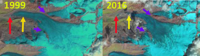
Landsat image sequence from 1999-2016.  Red arrows mark the 1999 terminus, yellow arrows the 2016 terminus and the purple arrow a tributary that detaches from Semitsiaq (S). Tasermiut Sermeq (T) retreats from the fjord. 

Tasermuit Fjord in southern Greenland is noted for its beauty, and until recently the fjord terminated at a glacier front. Currently no glacier reaches to the fjord. The retreat over the last two decades is similar to neighboring glaciers Kangersuneq Qingordleq and Qaleriq.  The loss of direct glacier connection is also occurring at Alangordlia. Here we examine Landsat images from 1999-2016 to observe glacier change. At the head of the fjord is Sermeq Tasermiut and on the east side is Sermitsiaq.

In 1999 the Sermitsiaq Glacier terminated at the eastern end of a small lake, red arrow.  Tasermiut Sermeq terminated in the fjord, red arrow.  By 2002 Sermitsiaq had retreated from the lake, while Tasermiut Sermeq still reached the fjord.  In 2013 Tasermiut Sermeq had retreated from the fjord and Sermitsiaq had retreated substantially from the lake and also had a significant tributary from the north detach, purple arrow. In 2016 Sermitsiaq has retreated 700 m since 1999, yellow arrow.  Biggs (2011) had noted a 610 m retreat of the glacier from 1987-2009, a slower rate than since 1999. Tasermiut Sermeq has retreated 300 m since 1999,and has a narrow steep tongue that will melt back quickly in the near future.

Murray et al (2015) examined 199 tidewater glaciers in Greenland and noted significant retreat of 188 of them. This is changing fjord dynamics, which will in the case of Tasermiut affect the marine biology, which has not been studied in any detail yet. Students on Ice 2014 Arctic Expedition provides exceptional imagery of this fjord and the Nanotarlik region.

tasermiut-ge-compare

Google Earth imagery of the region. illustrating the loss of fjord connection after 2009.

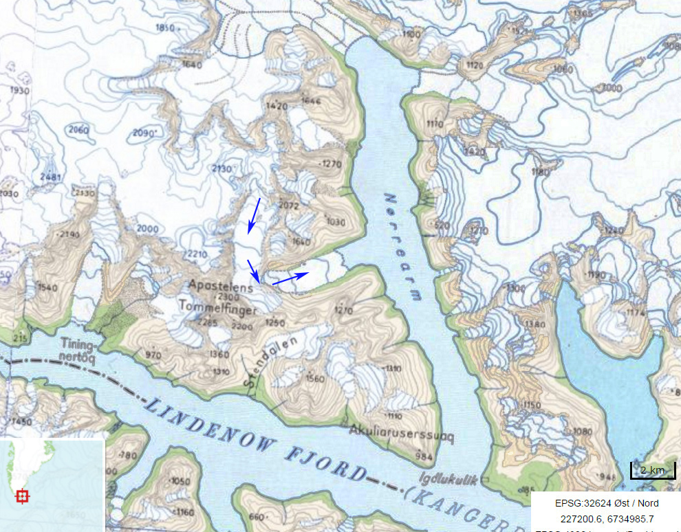
tasermiut-map

Map of the region 

Shatter & Shudder Glacier Retreat, British Columbia Lakes Form

shattter-terminus-compare

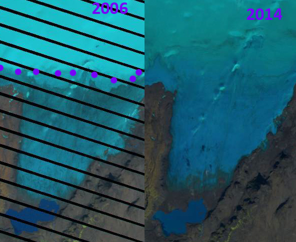
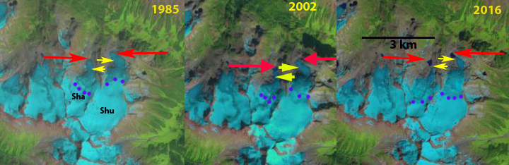
Red arrow is the 1985 terminus location and yellow arrow the 2016 terminus location.  Note the formatiion of new lakes at end of both glaciers. Purple dots is the transient snowline in August of each year.

Shatter and Shudder Glacier are at the eastern end of the Spearhead Range in Garibaldi Provincial Park, British Columbia. Osborn et al (2007) mapped the Little Ice Age extent of the glaciers compared to the 1990’s margins indicating a retreat of 300 m for Shatter Glacier and 700 m for Shudder Glacier (see below).  Koch et al (2009) identified the recession in area from 1928 to 1987 noting a 6% loss in Shatter Glacier and 22% loss for Shudder Glacier.  Koch et al (2009) identify an 18% loss in area from 1987-2005, indicating considerable recent change in the Park. Here we use Landsat imagery from 1985-2016 to update glacier change.

In 1985 there are no lake at the terminus of either Shatter or Shudder Glacier.  In 2002 a lake has formed at the terminus of Shudder Glacier, but not Shatter Glacier.  In 2016 both glaciers have proglacial lakes that have formed, and the terminus of both glaciers have retreated from the lakes.  This marks a retreat of 325 m on Shudder Glacier and 275 m on Shatter Glacier since 1985. Shudder Glacier retreated more rapidly in the first half of this period, while Shatter Glacier has experienced most of the retreat since 2005.

On Shatter and Shudder Glacier In 1987 the late August image indicates the snowline is at 2040 m, in mid-August 2015 the snowline is at 2250 m. In late August of 2014 the snowline was at 2120 m. In mid-August 2016 the snowline is at 2080 m. The higher snowlines are an indicator of mass loss for these glaciers that in turn drives retreat.  The region continues to experience significant loss in glacier area and development of many new alpine lakes with glacier retreat, five new lakes since 1987 just in this range with seven glaciers.  Spearhead and Decker Glacier are two other glaciers in the range that have developed new lakes since 1987. Nearby Helm Glacier is faring even worse.


shatter-tsl-compare

Landsat images from 1987, 2014 and 2015 indicating the transient snowline position at the purple dots on Shatter and Shudder Glacier.

spearhead-range-alpine-lakes-87-15

Pink Arrows indicate five new alpine lakes that have developed since 1987 as Spearhead Range glaciers have retreated

spearhead

Map of Spearhead Range glacier extent for LIA-Bold lines and 1987, light lines from Osborn et al (2007)

Findelengletscher, Switzerland Retreat & Hydrology Insights from David Collins

findelen compare

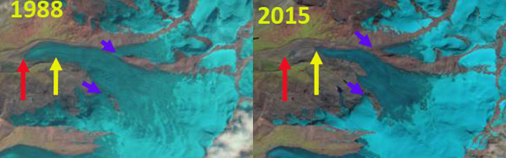
Landsat image comparison of Findelengletscher from 1988 to 2015. Red arrow indicating the 1988 terminus location and yellow arrow the 2015 terminus location.  The purple arrows indicate two tributaries connected to the main glacier in 1988 and now disconnected.

Findelengletscher along with Gornergletscher drains the west side of the mountain ridge extending from Lyskamm to Monte Rosa, Cima di Jazzi and Strahlhorn in the Swiss Alps.  It is the headwaters of the Matter Vispa.  This glacier was also the favorite field location for David Collins, British Glaciologist/Hydrologist from University of Salford who passed away last week. David had a wit, persistence and insight that are worth remembering. This post examines both David’s findings reaching back to the 1970’s gained from a study of glaciers in this basin and changes of the glacier since 1988 as evident in Landsat images. Findelengletscher drains into the Vispa River which supports for hydropower project, with runoff diverted into two hydropower reservoirs, Mattmarksee  operated by the Kraftwerke Mattmark producing 650 Gwh annually, and Lac de Dix operated by Grande Dixence that produces 2000 Gwh annually. There are two smaller run of river projects as well.

The Swiss Glacier Monitoring Network has monitored the terminus change of Findelengletscher since the 1890’s.  The glacier advanced 225 m from 1979-1986, retreated 450 m from 1988-1999 and retreated 850 m from 1999-2015. This is illustrated above with the red arrow indicating the 1988 terminus location and the yellow arrow the 2015 terminus location.  The purple arrows indicate two tributaries connected to the main glacier in 1988 and now disconnected.  The more limited retreated from 1988-1999 is evident in images below. The retreat is driven by mass losses with Huss et al (2012) noted as 1 m/year in the alps from 2001-2011. The snowline has typically been above 3250 m too high for equilibrium in the last decade. Melt at the terminus has typically been 7-8 m (WGMS).

Collins (1979) in work funded through hydropower looked at the chemistry of glacier runoff and found that glacier meltwater emerging in the outlet stream was enriched in Calcium, Magnesium and Potassium in particular versus non-glacier runoff, this led to a much higher conductivity. Collins (1982) noted the reduction in streamflow below Gornergletscher from summer streamflow events that reduced ablation for up to a week after the event. Collins (1998) noted that  a progressive rise of the transient snow line in summer increases the snow-free area, and hence the area of basin which rapidly responds to rainfall. Rainfall-induced floods are therefore most likely to be largest between mid-August and mid-September and in this period of warmer temperatures and higher snowlines. Collins (2002) Mean electrical conductivity of meltwater in 1998 was reduced by 40%. In the same 60 day period in 1998, however, solute flux was augmented by only 2% by comparison with 1979. Year-to-year climatic variations, reflected in discharge variability, strongly affect solute concentration in glacial meltwaters, but have limited impact on solute flux.  Collins (2006) identified that in highly glacier covered basins, over 60%, year-to-year variations in runoff mimic mean May–September air temperature, rising in the warm 1940s, declining in the cool 1970s, and increasing by 50% during the warm dry 1990s/2000s. In basins with between 35–60% glacier cover, flow also increased into the 1980s, but declined through the 1990s/2000s. With less than 2% glacier cover, the pattern of runoff was inverse of temperature and followed precipitation, dipping in the 1940s, rising in the cool-wet late 1960s, and declining into the 1990s/2000s.. On large glaciers melting was enhanced in warm summers but reduction of overall ice area through glacier recession led to runoff in the warmest summer (2003) being lower than the previous peak discharge recorded in the second warmest year 1947. Collins (2008)  examined records of discharge of rivers draining Alpine basins with between 0 and ∼70% ice cover, in the upper Aare and Rhône catchments, Switzerland, for the period 1894-2006  together with climatic data for 1866-2006 and found that glacier runoff had peaked in the late 1940s to early 1950s.

These observations have played out further with warming, retreat and more observations. Finger et al (2012) examine the impact of future warming on glacier runoff and hydropower in the region.  They observe that total runoff generation for hydropower production will decrease during the 21st century by about one third due glacier retreat. This would result in a decrease in hydropower production after the middle of the 21st century to keep Mattmarksee full under current hydropower production. Farinotti et al (2011) noted that the timing of maximal annual runoff is projected to occur before 2050 in all basins and that the maximum daily discharge date is expected to occur earlier at a rate of ~4 days/decade. Farinotti et al (2016) further wondered if replacing the natural storage of glacier in the Alps could be done with more alpine storage behind dams.

findelen

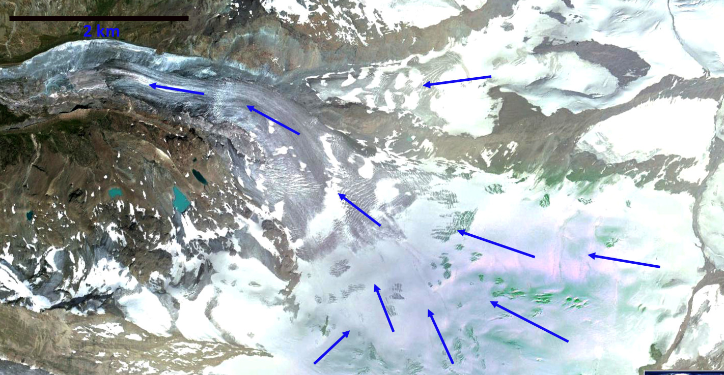
Google Earth image indicating flow of the Findelengletscher.

fiindelen 2 compare

Landsat image comparison of Findelengletscher from 1999 to 2016. Red arrow indicating the 1988 terminus location and yellow arrow the 2015 terminus location.  The purple arrows indicate two tributaries connected to the main glacier in 1988 and now disconnected.

Findelen terminus

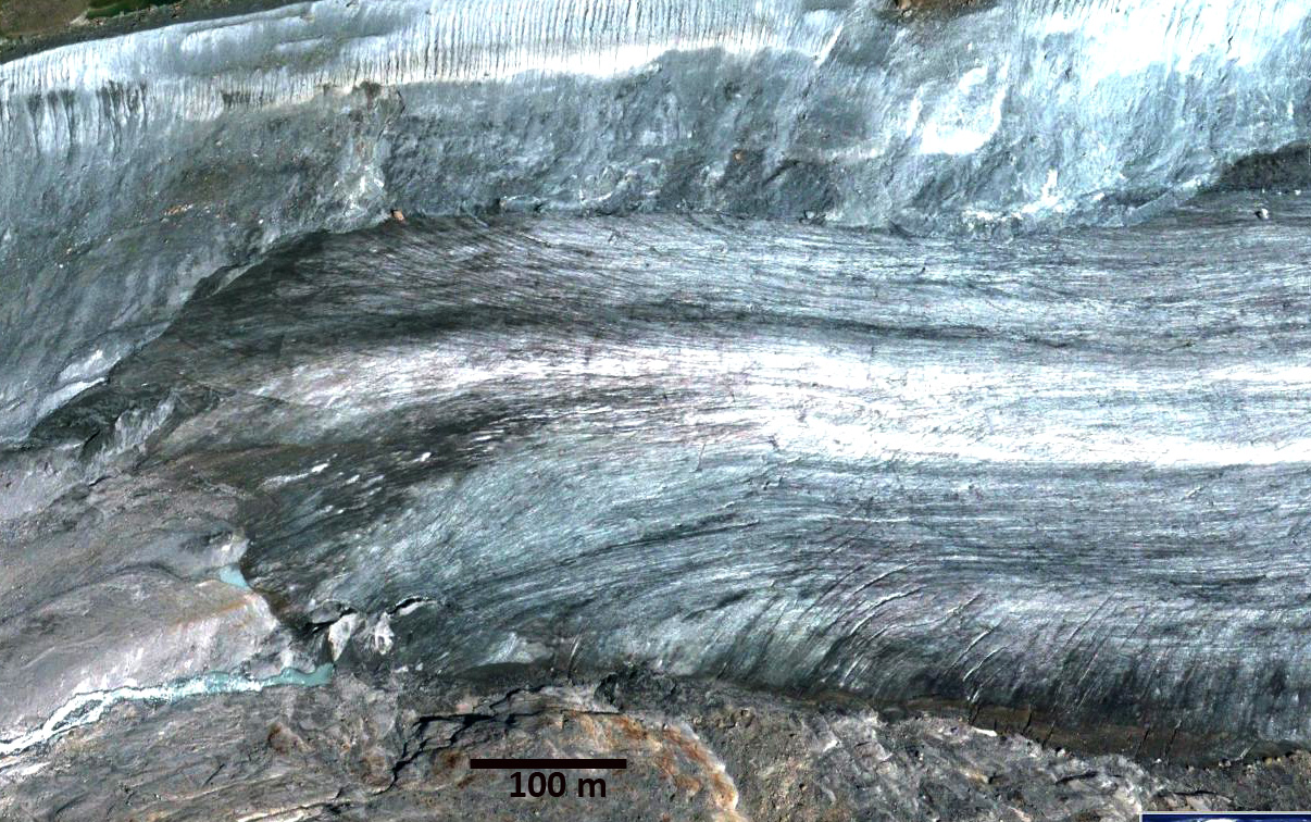
Terminus of Findelengletscher in Google Earth.  The lower several hundred meters has limited crevasses, but is not particularly thin. 


Storglombreen Glacier Loss, Norway

storg compare Landsat

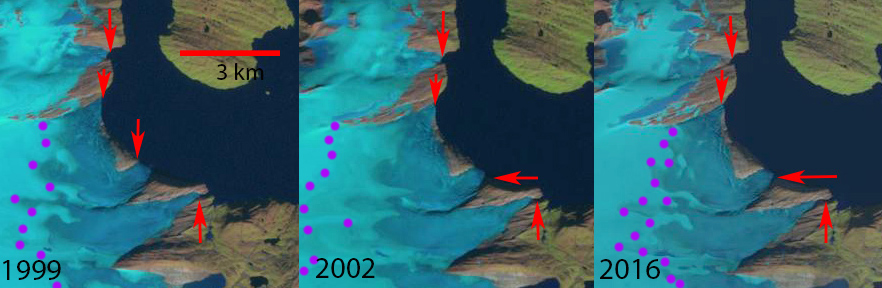
Landsat images from 199, 2002 and 2016 comparing glaciers draining into Storglomvatnet.  Red arrows indicate 1999 terminus locations, purple dots the snowline. 

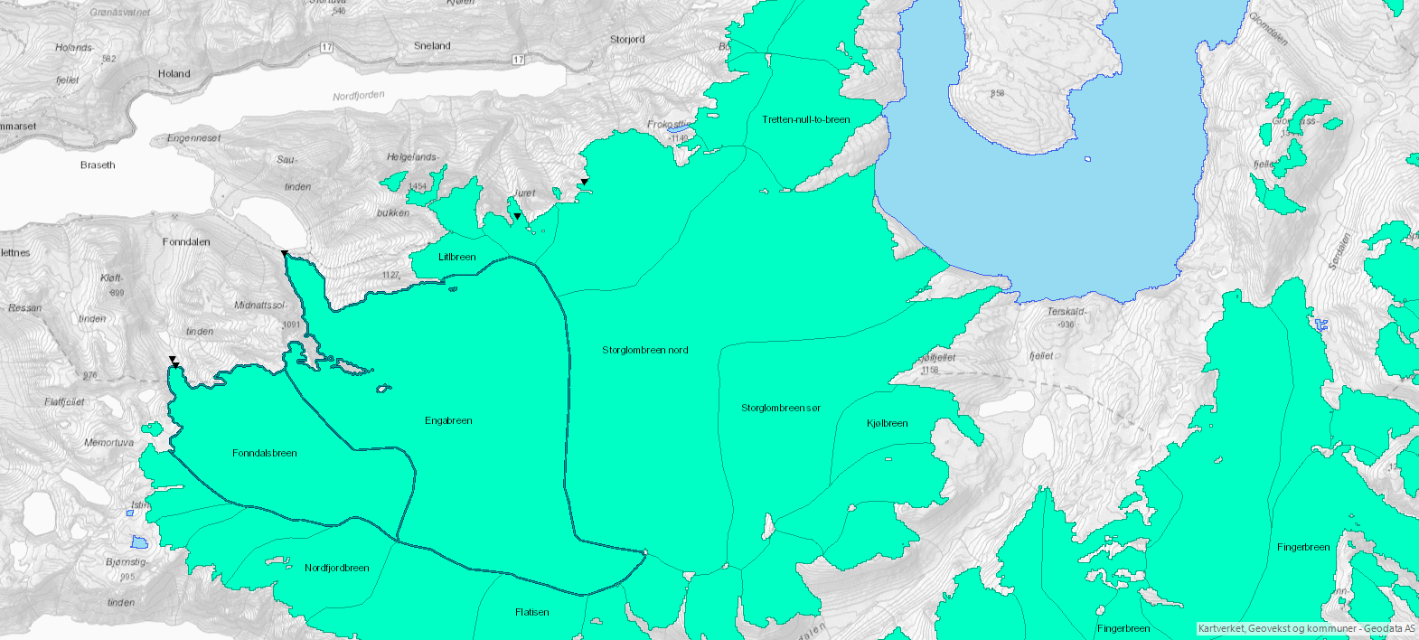
Storglomvatnet has several glacier that terminated in the lake in 1999, Storglombreen Nord, Sorglombreen Sud and Tretten. This lake is the main reservoir, 3.5 billion cubic meters that feeds the 350 MW Svartisen Hydropower plant. The lake has an elevation of 585 m, while the power plant is at sea level. Paul and Andreassen,(2009)  examined glacier area and found overall almost no areal extent change from 1968-1999 of Svartisen region glaciers, including the three examined here.  Engelhardt et al (2013), note this was due to positive trends of winter balance between 1961 and 2000, which have been followed by a remarkable decrease in both summer and winter balances leading to an average annual balance of –0.86±0.15 m w.e.a–1 between 2000 and 2010 .Since 1999 there have been changes. The Norwegian Glacier Inventory  and the online digital atlas use this 1999 imagery and indicate glacier area  for Storglombreen Sud at 15.9 km2, for Storglombreen Nord  at 41.2 km2 and Tretten-nulltobreen at 5.9 km2.

In 1999 each of the glaciers reaches the lake shore at 585 m in four separate terminus fronts. The snowline in 1999 is at 1150 m. In early August 2002 the termini still reach the lake shore and the snowline is higher at 1250 m.  In 2001, 2002 and 2003 mass balance measurements by the Norwegian Water Resources and Energy Directorate, indicate the snowline reached the top of the glacier at 1580 m. In 2016 the glacier termini no longer reach the lake shore and the snowline is again at 1150 m. It is evident in the Landsat image above that Storglombreen Sud and Tretten-nulltobreen no longer reach the lake shore, the southern most and northern most termini and arrows.  The two termini of Storglombreen Nord no longer reach the lake, though this requires higher resolution Sentinel 2 images to illustrate. Retreat of Tretten-nulltobreen from 1999-2016 has been 200 m, of Storglombreen Sud 250 m and of Storglmbreen Nord 100-200 m. There was limited calving into the lake and the retreat from the lake will not significantly alter the retreat rate of the glacier.  The high snowlines of recent years will lead to continued retreat. The retreat here is much less than on Engabreen which shares a divide with Storglombreen Nord, Flatisen  or Blåmannsisen.

svartisen west

Map of the glaciers in the region from the Norwegian Glacier Inventory online map application, based on 1999 images.

storg 2016 sentinel

Sentinel 2 image of the glaciers of Storglomvatnet from August 2016.  Notice that none of the termini reach the lake shore. 


Winsvold, Andreassen and Kienholz (2014)

Porcupine Glacier, BC 1.2km2 Calving Event Marks Rapid Retreat

porcupine iceberg comparison

Landsat images from Sept. 2015 and Sept. 2016.  Red arrow is the 1988 terminus and the yellow arrow the 2016 terminus.  I marks an icefall location and point A marks the large iceberg. 

Porcupine Glacier is a 20 km long outlet glacier of an icefield in the Hoodoo Mountains of Northern British Columbia that terminates in an expanding proglacial lake. During 2016 the glacier had a 1.2 square kilometer iceberg break off, leading to a retreat of 1.7 km in one year. This is an unusually large iceberg to calve off in a proglacial lake, the largest I have ever seen in British Columbia or Alaska. NASA has generated better imagery to illustrate my observations. Bolch et al (2010) noted a reduction of 0.3% per year in glacier area in the Northern Coast Mountains of British Columbia from 1985 to 2005. Scheifer et al (2007) noted an annual thinning rate of 0.8 meters/year from 1985-1999. Here we examine the rapid  retreat of Porcupine Glacier and the expansion of the lake it ends in from 1988-2016 using Landsat images from 1988, 1999, 2011, 2015 and 2016. Below is a Google Earth view of the glacier with arrows indicating the flow paths of the Porcupine Glacier. The second images is a map of the region from 1980 indicates a small marginal lake at the terminus.porcupine long term compare

Landsat images from 1988 and 2016 comparing terminus locations and snowline. Red arrow is the 1985 terminus and the yellow arrow the 2016 terminus.  I marks an icefall location and point A marks the large iceberg. Purple dots indicate the snowline.

In 1988 a tongue of the glacier in the center of the lake reached to within 1.5 km of the far shore of the lake, red arrow. The yellow arrow indicates the 2016 terminus position.  By 1999 there was only a narrow tongue reaching into the wider proglacial lake formed by the juncture of two tributaries. In 2011 this tongue had collapsed. In 2015 the glacier had retreated 3.1 km from the 1988 location.  In the next 12 months Porcupine Glacier calved a 1.2 square kilometer iceberg and retreated 1.7 km, detailed view of iceberg below. The base of the icefall indicates the likely limit of this lake basin. At that point the retreat rate will decline.The number of icebergs in the lake at the terminus indicates the retreat is mainly due to calving icebergs. Glacier thinning of the glacier tongue has led to enhanced calving. The retreat of this glacier is similar to a number of other glaciers in the area Great Glacier, Chickamin GlacierSouth Sawyer Glacier and Bromley Glacier. The retreat is driven by an increase in snowline/equilibrium line elevations which in 2016 is at 1700 m, similar to that on South Sawyer Glacier in 2016.porcupine 82716

August 27, 2016 Sentinel 2 image of iceberg red dots calved from front of Porcupine Glacier. 

porcupine glacier-map

Canadian Toporama map of Porcupine Glacier terminus area in 1980.

porucpine glacierge

Google Earth view indicating flow of Porcupine glacier.

porcupine glacier 1999

1999 Landsat image above and 2011 Landsat image below indicating expansion of the lake.  Red arrows indicate the snowline.  Purple, orange and yellow arrows indicate the same location in each image.

porcupine glacier bc 2011

South Sawyer Glacier Retreat and Separation, Alaska

south sawyer terminus compare

Comparison of South Sawyer Terminus position and unnamed glacier just to the south.  Red arrows are the 1985 terminus and yellow arrows the 2016 position of each terminus. 

South Sawyer Glacier is a 50 km long tidewater glacier terminating at the head of Tracy Arm fjord in Southeast Alaska.  The winding fjord surrounded by steep mountains is fed by Sawyer and South Sawyer Glacier is home to stellar sea lions, humpback whales and harbor seals.  This combination makes it attractive for cruise ships.  Mike Greenfelder a Naturalist/Photography Instructor with Lindblad Expeditions suggested I examine this glacier, and he provided several images. I had a chance to observe the glacier in 1982 and 1984 and noted that the snowline of the glacier at 1125 meters by Pelto (1987), using Landsat images.  We also identified the water depth at the glacier front was 180-200 m and the velocity of the calving front in the 1980’s was 1800 m/year (Pelto and Warren, 1990).  Today the velocity had declined  to less than half of this, which is expected given that water depth at the front in the most recent charts from 1999 indicate 1985 terminus position water depth is 110 m (Elliot et al, 2012). This is deep but not as deep as in the 1980’s, the greater the water depth, the greater the degree of buoyancy at the front and the higher the calving rate. The glacier retreated 3.5 km from 1899-1967 and then experienced little retreat from 1967 to 1985 (Molnia et al, 2008). Larsen et al (2007) observed a rapid thinning of the Stikine Icefield during the 1948-2000 period.The retreat has been driven by rising snowlines in the region that has driven the retreat of North Dawes, Baird, Dawes and Sawyer Glacier. Here we use Landsat images to indicate from 1985-2016 to identify terminus change and recent snowline elevation.

The terminus has retreated 2300 m from 1985 to 2016, with little retreat from 1985 to 1996.  Of equal importance is the glacier now appears to be near the tidewater limit of Tracy Arm.  In the gallery of terminus images below from Mike Greenfelder, the 2005 and 2012 images illustrate a sharp increase in slope at Point B and red arrows in 2015 just the red arrows, 300 m from the ice front.  In 2016 the ice front is nearly to the base of this icefall. This represents a sharp rise in the bed of glacier causing an icefall.  Whether the bed is entirely above sea level is not clear. Just south of the main terminus is a separate glacier that in 1985 was the combination of two tributaries.  By 2016 the two glaciers have separated with a retreat of  4.5 km for the western arm and 3.8 km for the eastern arm.

In the gallery of snowline images it is evident that upglacier there are two tributaries that joined the main glacier in 1985, that no longer reach the glacier in 2016.  This is indicative of the higher snowlines and thinning glacier. The gallery of snowlines  indicate the last date during the melt season with clear imagery of the snowline.  In 1985 the snowline was at 1250 m, in 1996 the snowline was at 1400 m, in 2013 1400 m, in 2014 1600 m, in 2015 at 1400 m and in 2016 at 1650 m.  The images are close to the end of the melt season, but are a minimum elevation for the equilibrium line.  The snowline is averaging 300 m higher than it did in the 1980’s. The retreat of South Sawyer Glacier and its iceberg production will slow as the water depth at the front declines in the near future.  The retreat will continue due to the sharp rise in snowlines that has occurred which has led to significant thinning up to 1500 m noted by Larsen et al (2007). The retreat of neighboring non-calving glaciers emphasizes this point.

[ngg_images source=”galleries” container_ids=”27″ display_type=”photocrati-nextgen_basic_imagebrowser” ajax_pagination=”1″ template=”/nas/wp/www/sites/blogsorg/wp-content/plugins/nextgen-gallery/products/photocrati_nextgen/modules/ngglegacy/view/imagebrowser-caption.php” order_by=”sortorder” order_direction=”ASC” returns=”included” maximum_entity_count=”500″]


World Glacier Monitoring Service 30th Anniversary

Zemp_20160831-25

The numbers on the left y-axis depict quantities of glacial mass loss from the WGMS and sea level rise, and the suns across the horizon contain numbers that represent the global increase in temperature, coinciding with the timeline on the lower x-axis From Jill Pelto

The World Glacier Monitoring Service (WGMS) celebrated 30 years of achievement last week. I have had the privilege of being the United States representative to the WGMS and was an invited speaker for the Jubilee held in Zurich, Switzerland along with Matthias Huss, Wilfried Haeberli, Liss Marie Andreassen and Irene Kopelman. This post examines the important role that WGMS has and continues to serve under the leadership of Michael Zemp. The organization has been compiling, homogenizing and publishing data on glacier fluctuations and mass balance primarily from 1986-2013. WGMS remains the leading organization for the collection, storage and dissemination of information on the fluctuations of alpine glaciers. The resulting standardized collection of alpine glacier data that is archived by WGMS, is also leading to analysis efforts that otherwise would be hampered by limited data and lack of homogeneity to the data. Glaciers are recognized as one of the best climate indicators.  Mass balance data is the best parameter to measure on glaciers for identifying climate change, because of its annual resolution. The core of the WGMS data set has been frontal variations, which indicate longer response to climate as well as dynamic changes.  The key data set today provided by WGMS are the reference glaciers.

This set of glaciers has a 30-year continuous record of annual mass balance measured in the field, and each glacier also has geodetic verification.  This mass balance data set is featured on the Global Climate Dashboard at NOAA. I report the mass balance of two reference glaciers Lemon Creek Glacier in Alaska and Columbia Glacier in Washington.  Today the field based work is being increasingly supplemented and supplanted by remote sensing methods.  This data sets indicates a period of sustained mass balance loss, and glacier retreat that Zemp et al (2015) using WGMS data noted as historically unprecedented.  The most recent compilation publication is the Global Glacier Change Bulletin.

This data set is of particular value during this period of climate change and is already chronicling the disapperance of a number of glaciers in the data set. Glacier loss is not a process that has been well documented. The WGMS data set can be enriched by more data from expanding monitoring, reporting data from archives and simply adding the submission of data as a step in the research process for those monitoring alpine glaciers. The video of my presentation looking at 33 consecutive years of field work and sharing this data after compilation with the WGMS is below. The slides below are from the Jubilee presentations.


[ngg_images source=”galleries” container_ids=”32″ display_type=”photocrati-nextgen_basic_imagebrowser” ajax_pagination=”1″ template=”/nas/wp/www/sites/blogsorg/wp-content/plugins/nextgen-gallery/products/photocrati_nextgen/modules/ngglegacy/view/imagebrowser-caption.php” order_by=”sortorder” order_direction=”ASC” returns=”included” maximum_entity_count=”500″]

Moulins: Clarifying Impacts on Glacier Velocity

In the last week I have read three separate articles referring to glacier moulins as lubricating the bed of a glacier resulting in overall velocity increase, for example EOS (Aug. 2016), this is not generally accurate. Having spent considerable time observing moulins and reviewing some excellent studies that indicate their impact, it is worth noting again a more complete picture of the role moulins play.  This is a role that warrants considerable further examination. In 2008 and 2011 I wrote a piece indicating why this a generalization that is only sometimes accurate.  The key to increasing glacier velocity is high basal water pressure, not simply lots of meltwater.  Think of your car, if you have low oil pressure that is an issue for efficient running.  If you have high oil pressure that is ideal.  If you have high oil pressure and you add more oil that does not further lubricate the engine.  Delivering more water to the base of a glacier that already has lots of meltwater drainage will not typically lead to a significant acceleration.  A number of studies since 2008 have better illustrated this principle as it applies to ice sheets.

Ahlstrøm et al (2013) examined 17 Greenland glaciers and noted a pattern, “Common to all the observed glacier velocity records is a pronounced seasonal variation, with an early melt season maximum generally followed by a rapid mid-melt season deceleration”.  This indicates the Greenland glaciers are more like a typical alpine glacier and are susceptible to the forces that tend to cause alpine glaciers to experience peak flow during spring and early summer.  Those forces are the delivery of meltwater to the base of the glacier, when a basal conduit system is poorly developed.  This leads to high basal water pressure, which enhances sliding.  As the conduit system develops/evolves the basal water pressure declines as does basal sliding, even with more meltwater runoff.

This is what has been reported to be the case by Sundal et al (2011) in Greenland.  They found a similar early season velocity in all years, with a reduced velocity late in summer during the warmest years.  This suggested that a more efficient melt drainage system had developed, reducing basal water pressure for a longer period of time. The meltwater lubrication mechanism is real, but as observed is limited both in time and area impacted.  It is likely that, as on alpine glaciers, the seasonal speedup is offset by a greater slowdown late in the melt season.  Most observed acceleration due to high meltwater input has been on the order of several weeks, leading to a 10-20% flow increase for that period.

Moon et al (2014) examined 55 Greenland glaciers and found three distinct seasonal velocity patterns. Type 1 behavior is characterized by speedup between late spring and early summer with speed remaining high until late winter or early spring, with the principal sensitivity being to terminus conditions and position. Type 2 behavior has stable velocity from late summer through spring, with a strong early summer speedup as runoff increases and midsummer slowing, as the glacier develops an efficient drainage system.  Type 3 behavior has a mid-summer slowdown leading to a pronounced late summer minimum during the period of maximum runoff.  Velocity than rebounds over the winter.  The common behavior is then a slowdown during periods of peak runoff and moulin drainage.

Anderson et al (2011) noted that changes in velocity due to a 45% change in meltwater input were small 4-5% on Helheim Glacier.

Clason et al (2015) modelled development of moulins and their ability to deliver the water to the bed of Leverett Glacier.  This study illustrates the level of details that is being examined to better model meltwater routing, which will inform flow models as noted by EOS (2015).

Moulins increase meltwater flow to a glacier bed.  In areas where significant surface melt occurs, this tends to lead to an early melt season increase in basal water pressure and then velocity.  This is typically followed by a mid/late melt season deceleration with continued meltwater drainage through moulins.  The lubrication is hence, restricted in time, and if followed by a deceleration, does not necessarily lead to an increase in the overall glacier velocity.  Certainly in some cases moulins will increase overall velocity and in others not.

Lednikovoye Glaciers, Novaya Zemlya 1999-2016 retreat

lenikovoye compare

Comparison of glaciers terminating in Lednikovoye Lake in central Svalbard in 2000 and 2016. Red arrow is the 2000 terminus location and yellow arrows the 2016 terminus location.

Lednikovoye Lake in central Novaya Zemlya has four glaciers terminating in it. Here we examine the two unnamed glaciers that discharge into the northwest portion of the lake. The glaciers are retreating like all tidewater glaciers in northern Novaya Zemlya, though they are not specifically tidewater (LEGOS, 2006). LEGOS (2006) identified a 2.7 square kilometer reduction in area of the two glaciers from 1990-2000.  Carr et al (2014) identified an average retreat rate of 52 meters/year for tidewater glaciers on Novaya Zemlya from 1992 to 2010 and 5 meters/year for land terminating glaciers.Here we use Landsat images to examine changes from 1999 to 2016.

In 1999 and 2000 the western Lednikovoye Glacier ended on an island, the eastern Lednikovoye Glacier extended past the exit of a glacier filled valley entering from the east.  By 2016 the western terminus had retreated 800 meters from the newly developed island.  The eastern terminus had retreated a similar amount now ending near the center of the valley entering on the east.  The glacier in that eastern valley has retreated 600 m from 1999 to 2016. The snowline in 2000 and 2016 is at ~500 m, with a significant remaining accumulation zone.  There is limited upglacier thinning suggesting that retreat will not become rapid.  The reduced rate of retreat of the Lednikovoye Glacier’s versus tidewater glacier of Novaya Zemlya suggests the importance of both sea ice reduction and sea surface temperature increase to the retreat rate of the latter such as Krayniy Glacier, Tasija Glacier and Chernysheva Glacier.

ledknikovoye 1999

lednikovoye 2015

Looking Inside a Glacier

Here we provide a visual look inside a glacier in the North Cascades of Washington.  Glaciers are not all the same, but the key internal ingredients in summer typically are in varied ratios: ice, meltwater, sediment and biologic material.  In this case there are torrents of water pouring through the interior of the glacier, generated at the surface the day we are filming.  We do measure the discharge and velocity of these streams.  Once they drain englacially they are much slower as there are numerous plunge pools.  There are also plenty of water filled crevasses. Some of the streams have considerable sediment in them, usually large clasts given the high velocity and low bed friction.  In this case there are also a great many ice worms clinging to the walls of a water filled crevasse, and the walls of the stream channels.  All of this water than merges by the terminus into an outlet stream.  This again we measure.  On the glacier we are measuring melt and at the end of the glacier runoff provides an independent measure of this melt as well. The water then heads downstream supplying many types of fish enroute to the ocean.

The last three years have led to considerable mass loss of glaciers in the area.  This means less snowcover at the surface, which leaves less room for the ice worms to live and forces them into the meltwater regions.  This also leads to more supraglacial stream channels, which develop and deepen.  In many cases the streams deepen to the point that they become englacial. The increased ice area also should stress glacier ice worms as they live on algae, which resides largely in snow, which is less extensive and persistent in recent summers.

Glaciers in BAMS State of Climate 2015

Decrease in Glacier Mass Balance uses measurements from 1980-2014 of the average mass balance for a group of North Cascade, WA glaciers. Mass balance is the annual budget for the glaciers: total snow accumulation minus total snow ablation. Not only are mass balances consistently negative, they are also continually decreasing. Glaciers have been one of the key and most iconic examples of the impact of global warming.  

BAMS State of Climate 2015 asked me about featuring some of the glacier images for the cover, and I countered with a suggestion to utilize one of a series of paintings by Jill Pelto that illustrate the impact of climate change magnifying the impact of the data.  Below are sections of this years report that focus on glaciers.

Glaciers and ice caps (outside Greenland)

M. Sharp, G. Wolken, L.M Andreassen, A. Arendt, D. Burgess, J.G. Cogley, L. Copland, J. Kohler, S. O’Neel, M. Pelto, L.Thompson, and B. Wouters

Among the seven glaciers for which 2014-2015 annual mass balance have been reported, the mass balances of glaciers in Alaska and Svalbard (three each) were negative, while the balance for Engabreen Glacier in Norway was positive. The pattern of negative balances in Alaska and Svalbard is also captured in time series of regional total stored water estimates, derived using GRACE satellite gravimetry, which are a proxy for regional total mass balance (ΔM) for the heavily glacierized regions of the Arctic (Figure 3). Measurements of ΔM in 2014-2015 for all the glaciers and ice caps in Arctic Canada and the Russian Arctic also show a negative mass balance year. The GRACE-derived time series clearly show a continuation of negative trends in ΔM for all measured regions in the Arctic. These measurements of mass balance and ΔM are consistent with anomalously warm (up to +1.5ºC) summer air temperatures over Alaska, Arctic Canada, the Russian Arctic, and Svalbard in 2015, and anomalously cool temperatures in northern Scandinavia, particularly in early summer (up to -2ºC). The warmer temperatures led to higher snowlines in the aforementioned regions as seen in images below.

clephane bay compare

Baffin Island Ice Cap near Clephane Bay indicate limited snowpack in 2015

frostisen compare

Frostisen Ice Cap, Svalbard with limited 2015 snowpack.

Alpine Glaciers

M.Pelto

Preliminary data for 2015 from 16 nations with more than one reporting glacier from Argentina, Austria, Canada, Chile, Italy, Kyrgyzstan, Norway, Switzerland, and United States indicate that 2015 will be the 32nd consecutive year of negative annual balances with a mean loss of -1169 mm for 33 reporting reference glaciers and -1481 mm for all 59 reporting glaciers. The number of reporting reference glaciers is 90% of the total whereas only 50% of all glaciers that will report have submitted data thusfar. The 2015 mass balance will likely be comparable to 2003, the most negative year at -1268 mm for reference glaciers and -1198 mm for all glaciers.

The cumulative mass balance loss from 1980-2015 is 18.8 m, the equivalent of cutting a 20.5 m thick slice off the top of the average glacier (Figure 1).  The trend is remarkably consistent from region to region (WGMS, 2015).  The decadal mean annual mass balance was -261 mm in the 1980’s, -386 mm in the 1990’s, 727 mm for 2000’s and -818 mm from 2010-2015.  The declining mass balance trend during a period of retreat indicates alpine glaciers are not approaching equilibrium and retreat will continue to be the dominant terminus response (Zemp et al., 2015). The recent rapid retreat and prolonged negative balances has led to many glaciers disappearing and others fragmenting (Pelto, 2010; Carturan et al, 2015).

columbia compare

In South America seven glaciers in Columbia, Argentina and Chile reported mass balance. All seven glaciers had losses greater than 1200 mm, with a mean of -2200 mm.  These Andes glaciers span 58 degrees of latitude.

In the European Alps, mass balance has been reported for 14 glaciers from Austria, France, Italy and Switzerland.  All 14 had negative balances exceeding 1000 mm, with a mean of -1865 mm. This is an exceptionally negative mass balance rivaling 2003 when average losses exceeded -2000 mm.

In Norway mass balance was reported for six glaciers in 2015, all six were positive with a mean of 780 mm.  This is the only region that had a positive balance for the year. In Svalbard six glaciers reported mass balances, with all six having a negative mass balance averaging -675 mm.

In Alberta, British Columbia, Washington and Alaska mass balance data from 17 glaciers was reported with a mean loss of -2590 mm, with all 17 being negative. This is the most negative mass balance for the region during the period of record.  From Alaska south through British Columbia to Washington the accumulation season temperature was exceptional with the mean for November-April being the highest observed.

In the high mountains of central Asia six glaciers from Russia, Kazakhstan, and Kyrgyzstan reported data, all were negative with a mean of -660 mm.

Columbia Glacier having lost nearly all of its snowcover by early August had its most negative mass balance of any years since measurements began in 1984