From a Glaciologists Perspective AGU Day 1

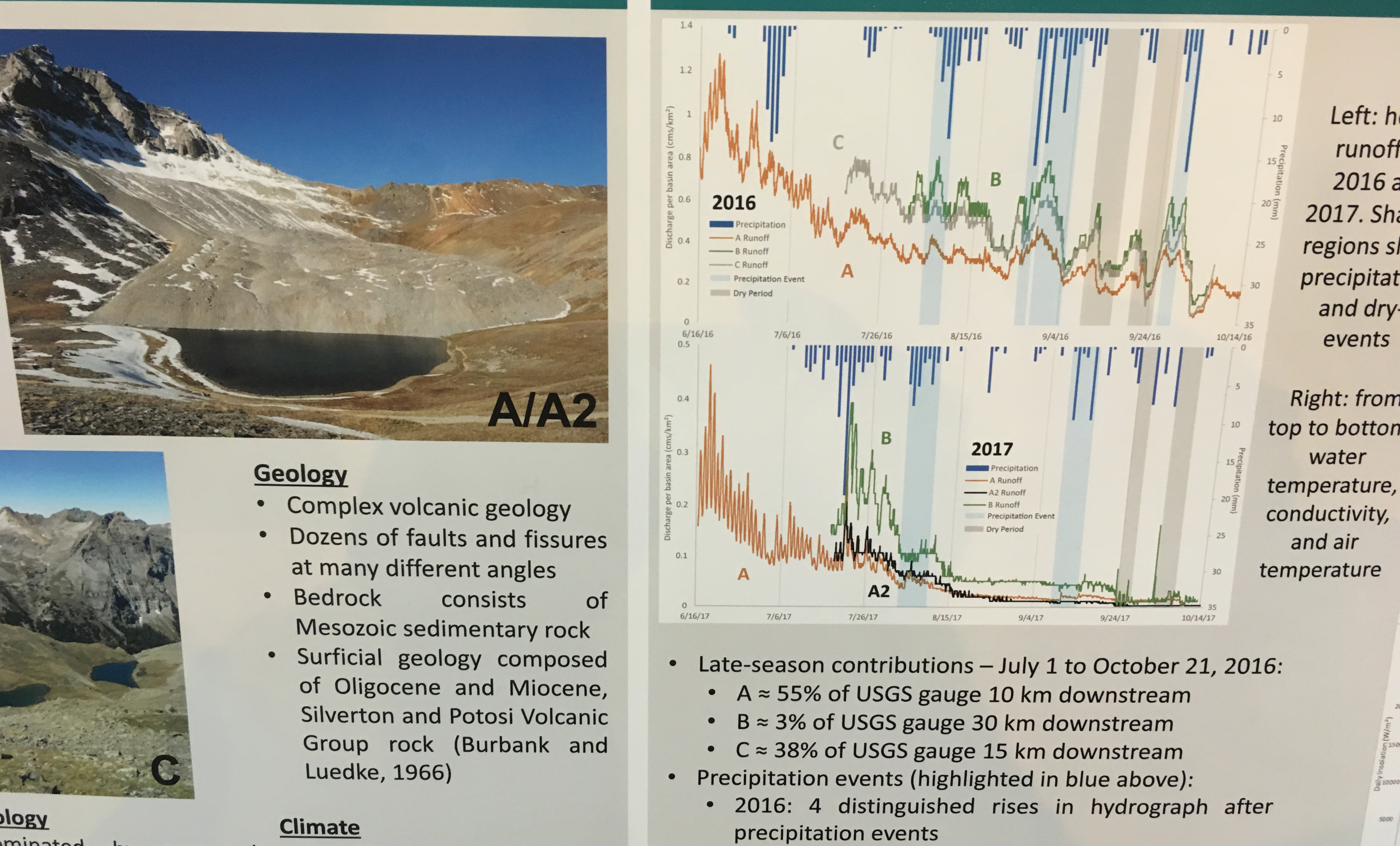
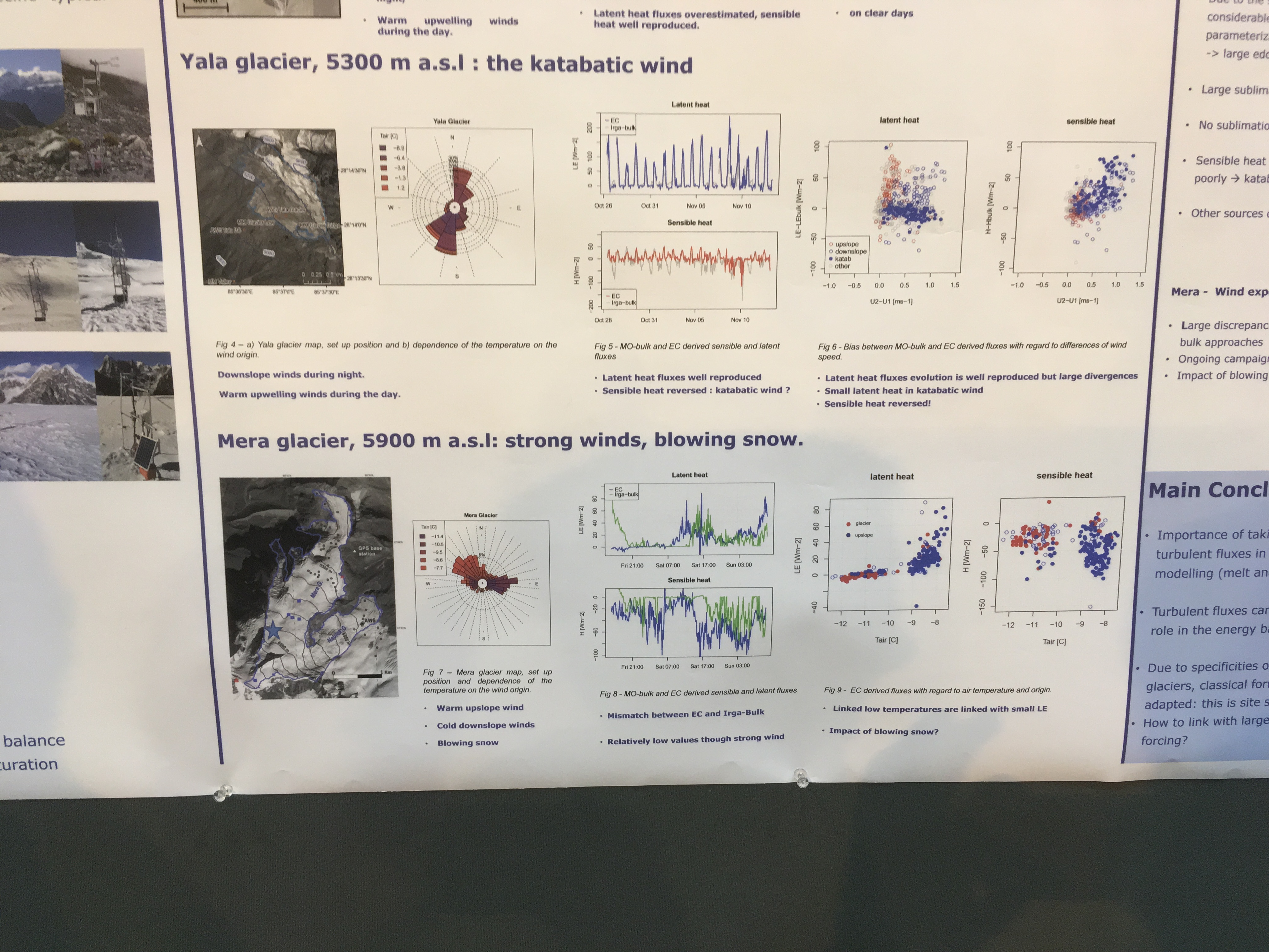
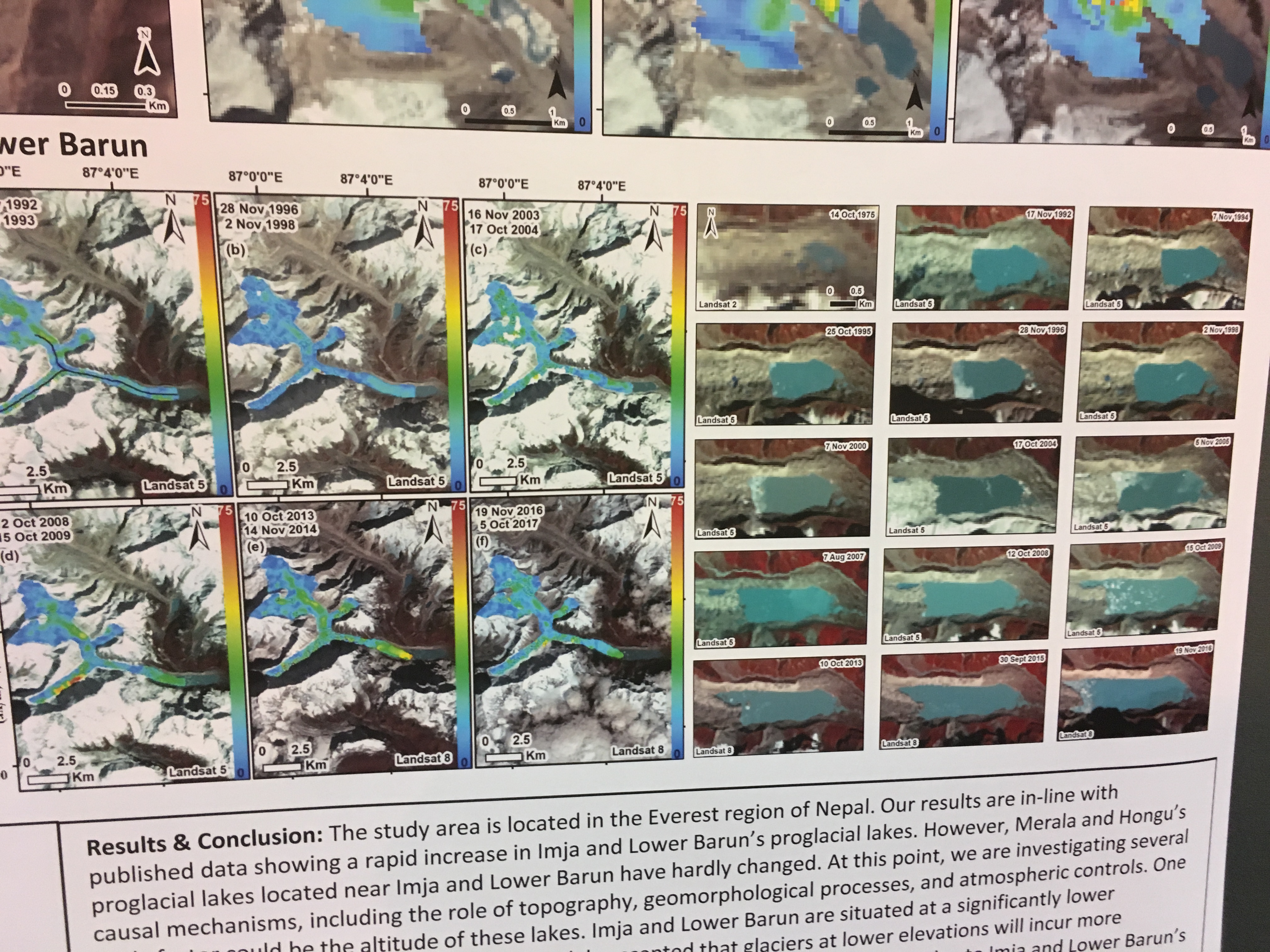
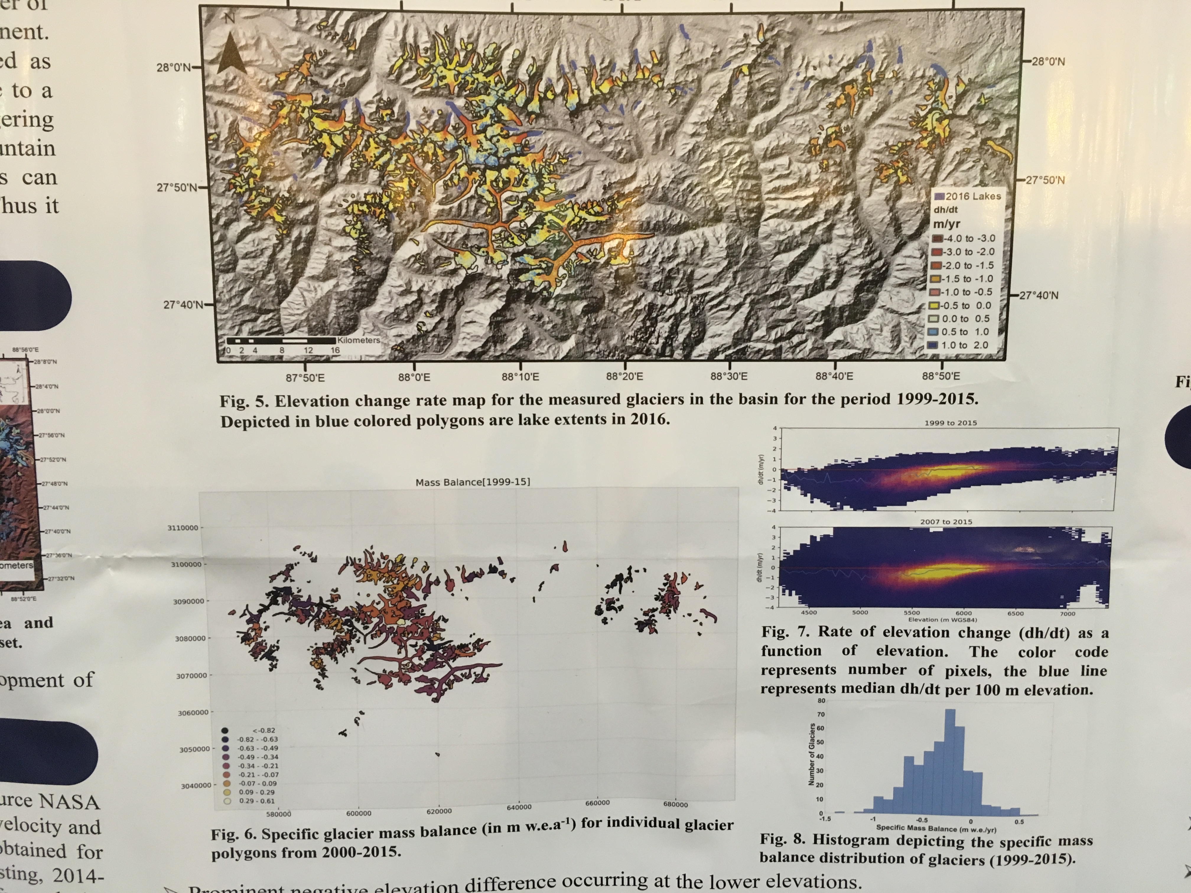
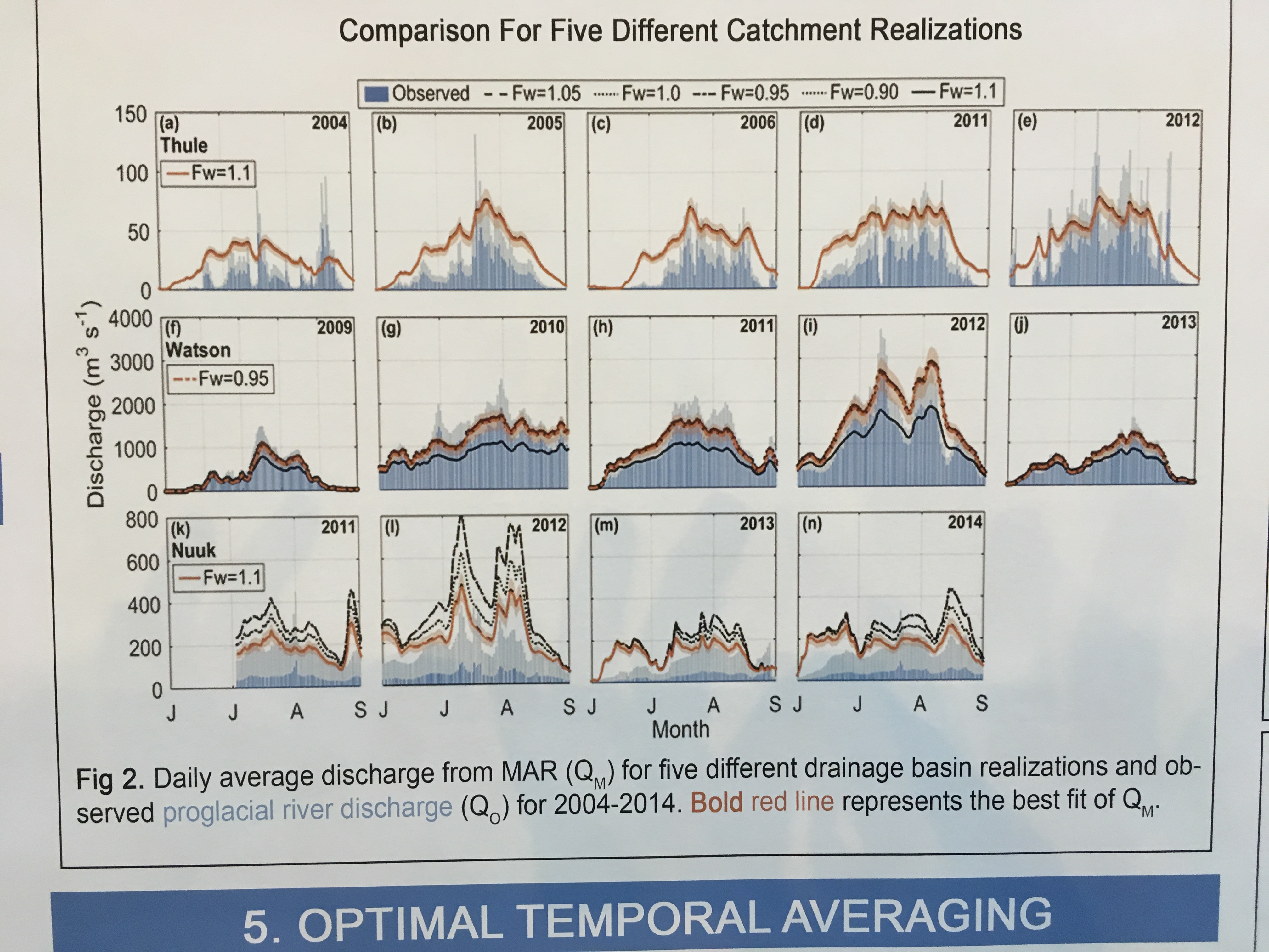
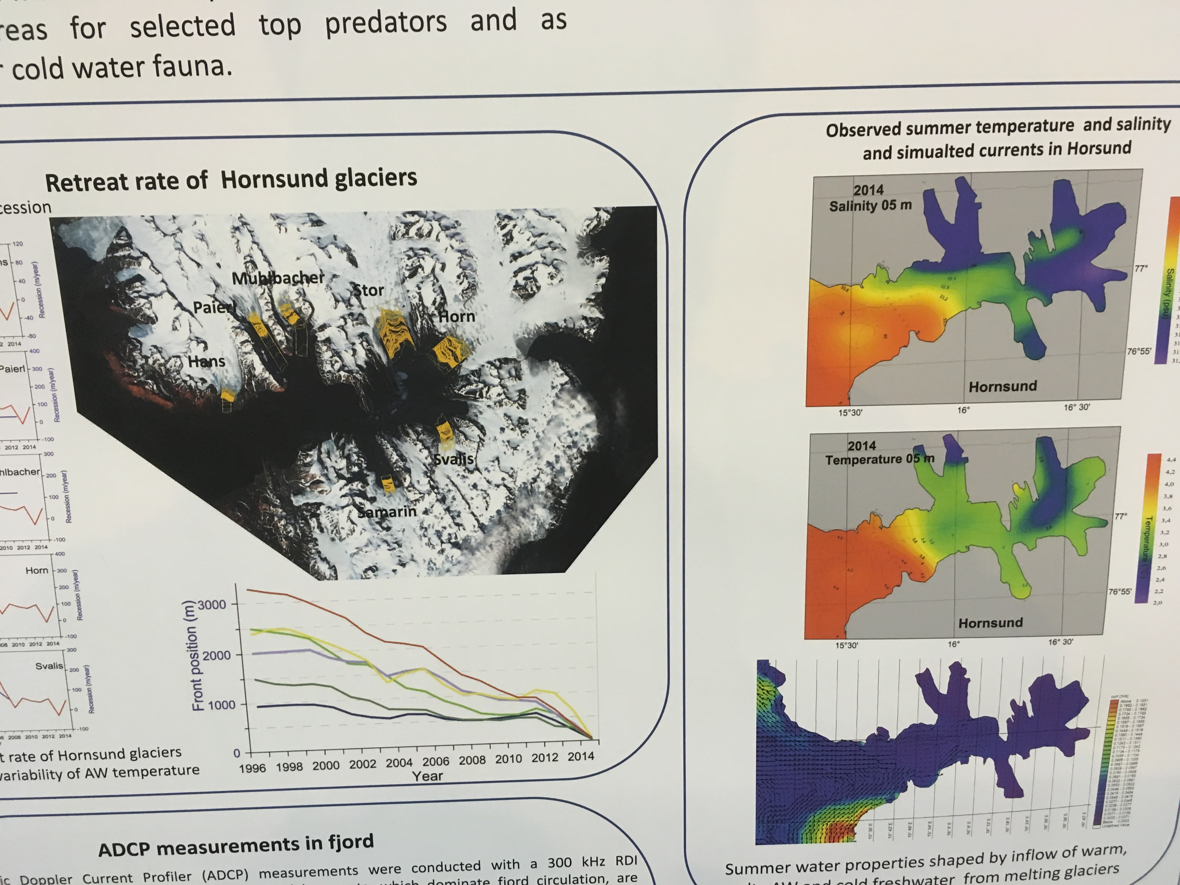
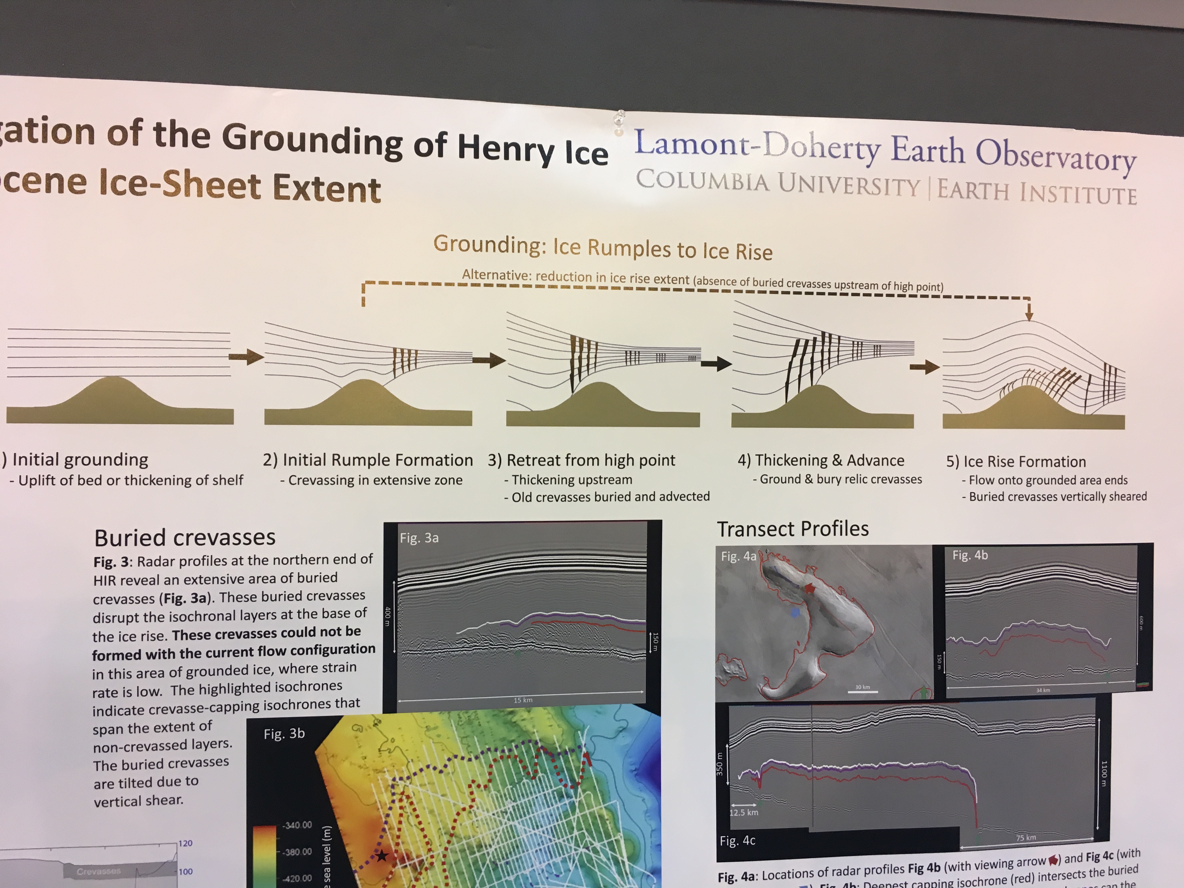
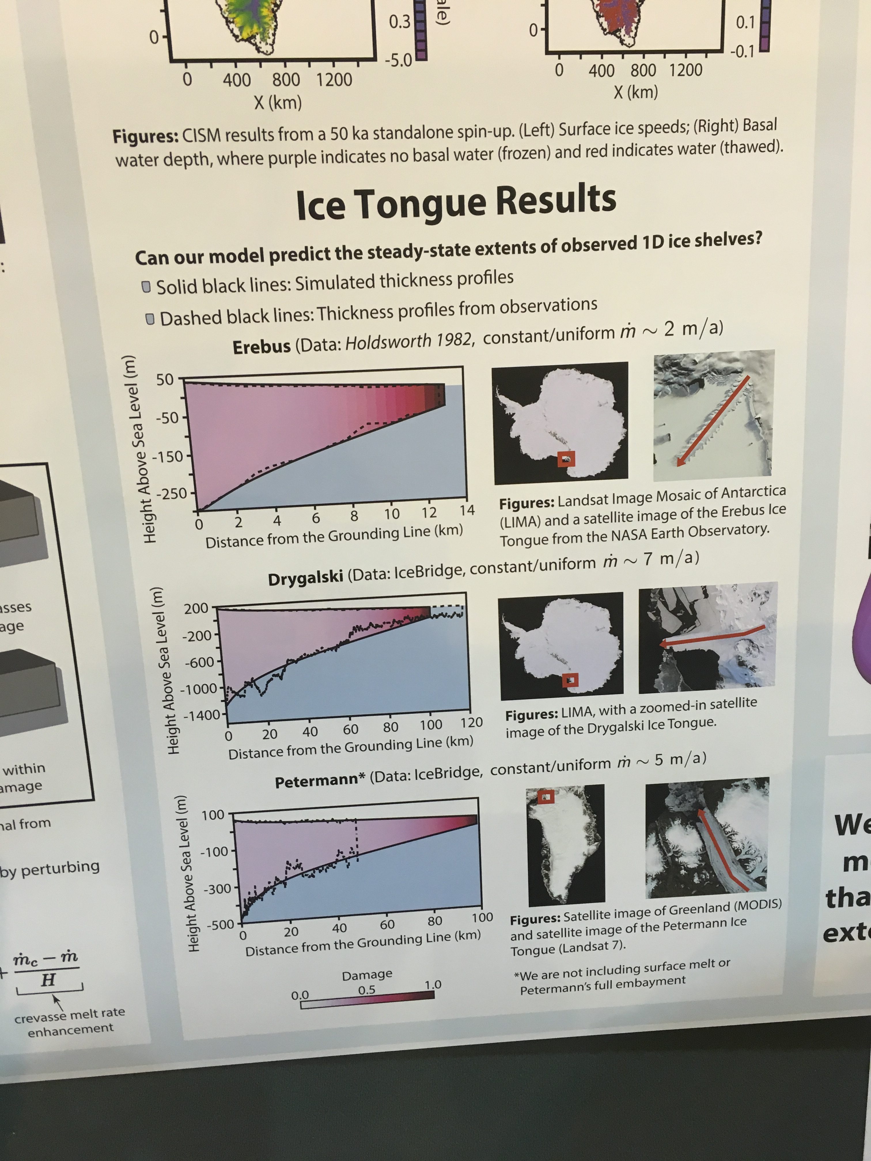
The theme changes from a glaciers to a glaciologists perspective with a focus on selected work at the AGU 2017. The research discussed here is from the Poster Paper sessions the most interactive part of the convention.  The following are some interesting snapshots of the breadth and depth of ongoing research.  The most compelling figure from each poster is used.

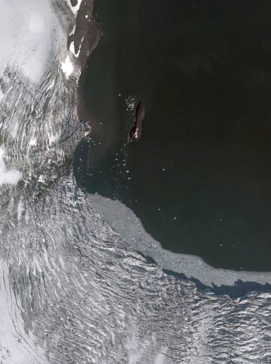
Richard Forster, U of Utah team presented work on the firn aquifer in Greenland.  A feature we did not even know existed until 2011. They have conducted four field seasons,  using ground penetrating radar  and magnetic resonance soundings to map water table elevation, thickness and volume in several areas.  They found the aquifer thickness has a typical thickness of 10-30 m.  Further they found that firn aquifers have existed since at least 1993 and have expanded and shifted with time see above image.

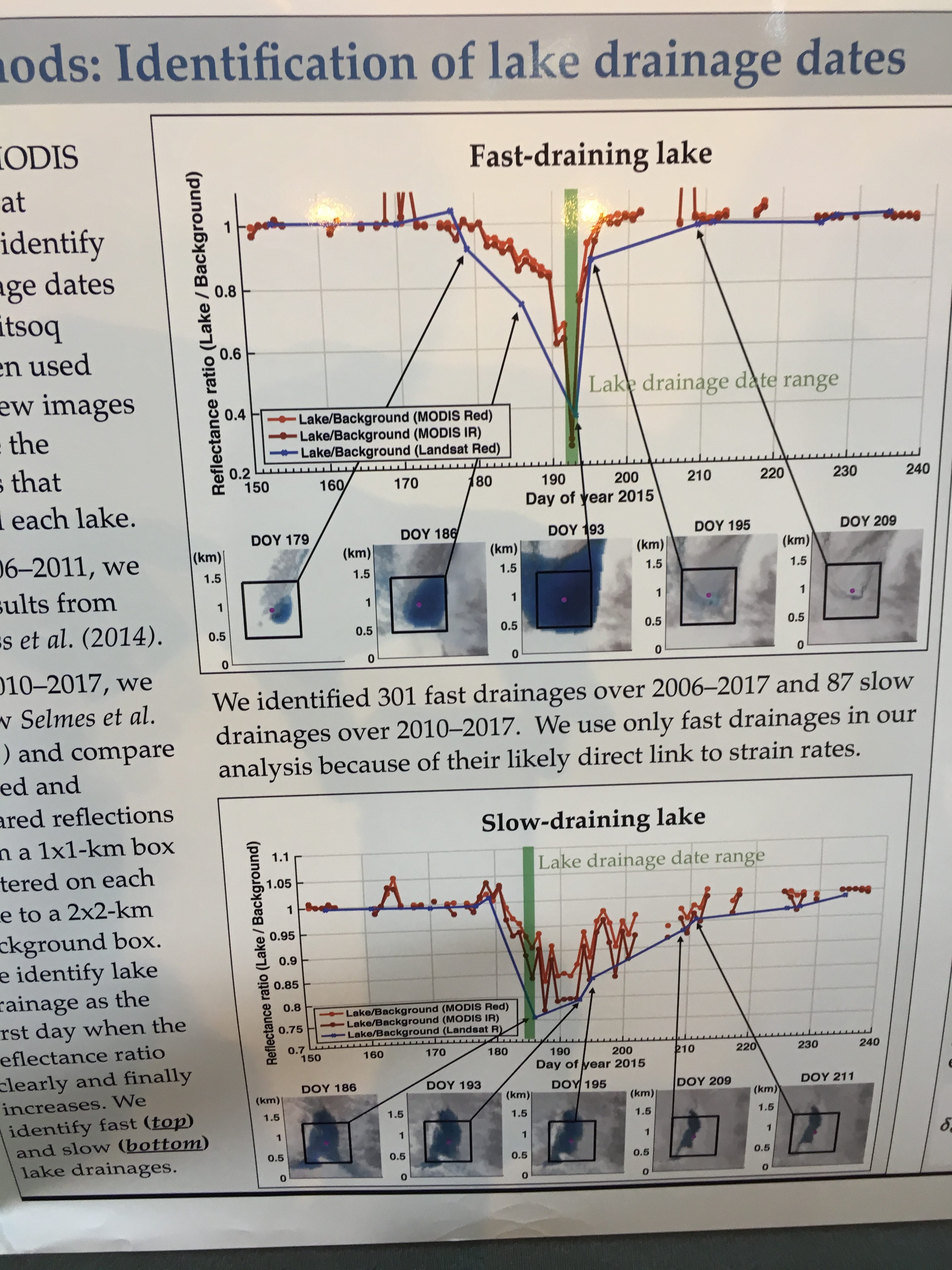
Kristin Poinar, NASA GSFC team examined the drainage of supraglacial lakes in Greenland. They investigated factors that control when and where the lakes drain to the ice sheet base. They observed  359 lake drainage events in a west Greenland region and compare the dates of these drainage events to strain rates calculated from satellite data. They noted both slow draining and fast draining lakes, the faster drainages occurring later in the summer on average. They found that strain rates did not satisfactorily predict lake drainage date.  

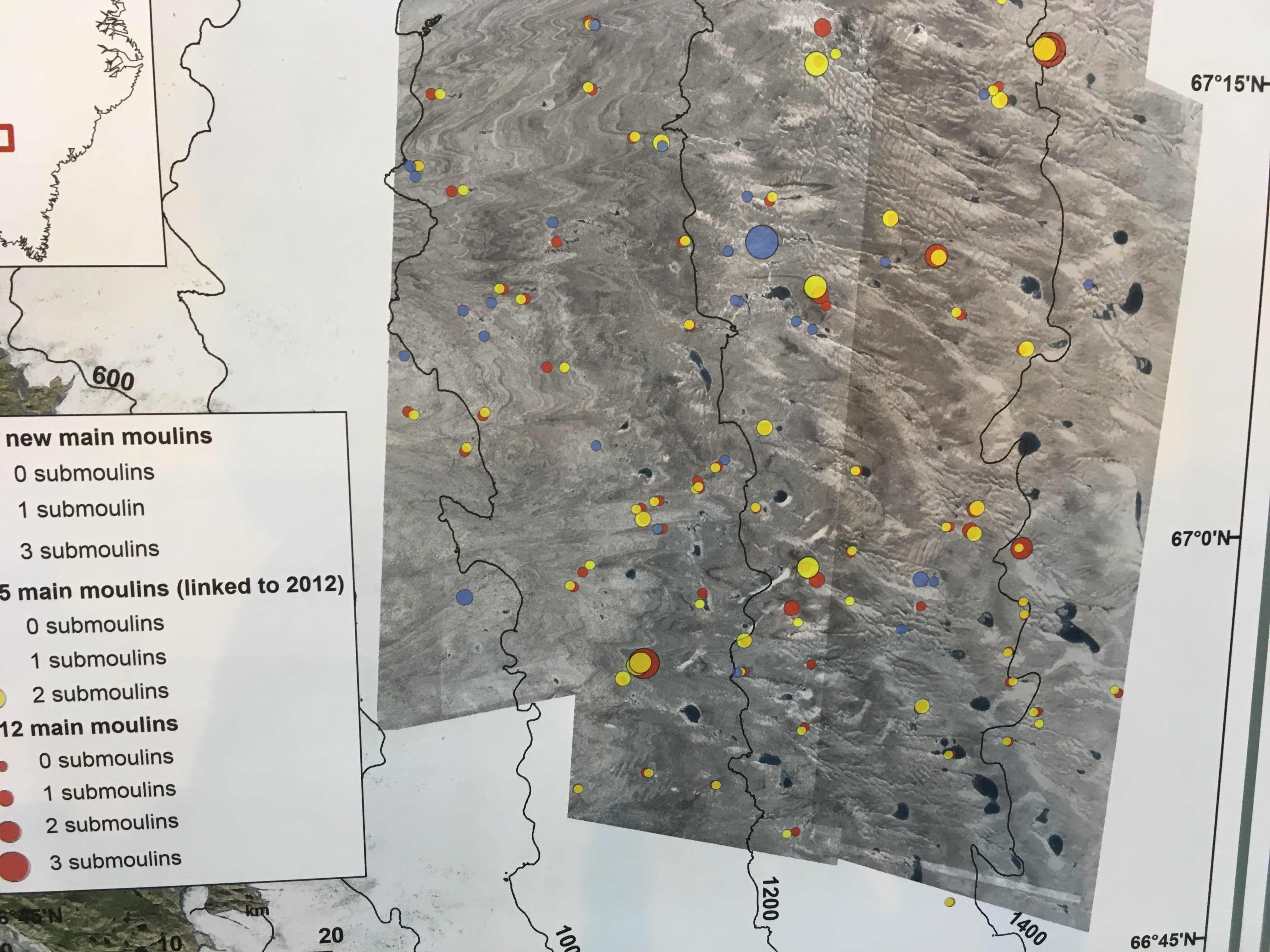
Vena Chu at UC-Santa Barbara’s team mapped river networks On Russell Glacier that terminate into moulins which connect surface melt to englacial and subglacial drainage networks. They used WorldView imagery to show development of molins and their migration between 2012 and 2015.   The majority of moulins they mapped in 2015 were  moulins in 2012. New moulins most commonly formed in crevassed, thinner ice areas near the ice margin, and a lesser but significant quantity at higher elevations above 1300 m.

Rohi Muthyala, Rutgers University team measured the discharge of supraglacial streams for three months, constructing rating curves.  They compared air temperature and discharge in the upper and lower basin.  The upper basin was more related to the daily air temperature. The stream system feeds into a moulin system.

Mariah Radue, University of Maine’s team mapped and dated the moraines and erratics adjacent to Potanin Glacier in the Mongolian Altai (49°N, 88°E). They used 10Be surface-exposure chronology to date glacial landforms mapped using satellite and Drone imagery. Based on our glacial reconstruction, we estimate changes in atmospheric temperature from the Last Glacial Maximum to the Late Holocene using snowline reconstruction techniques. Mongolia is a unique location because it is isolated from oceanic influences and a climate could provide insight into the roles of local radiation forcing from earth orbital changes, greenhouse gases, and a Asian climate dynamics.

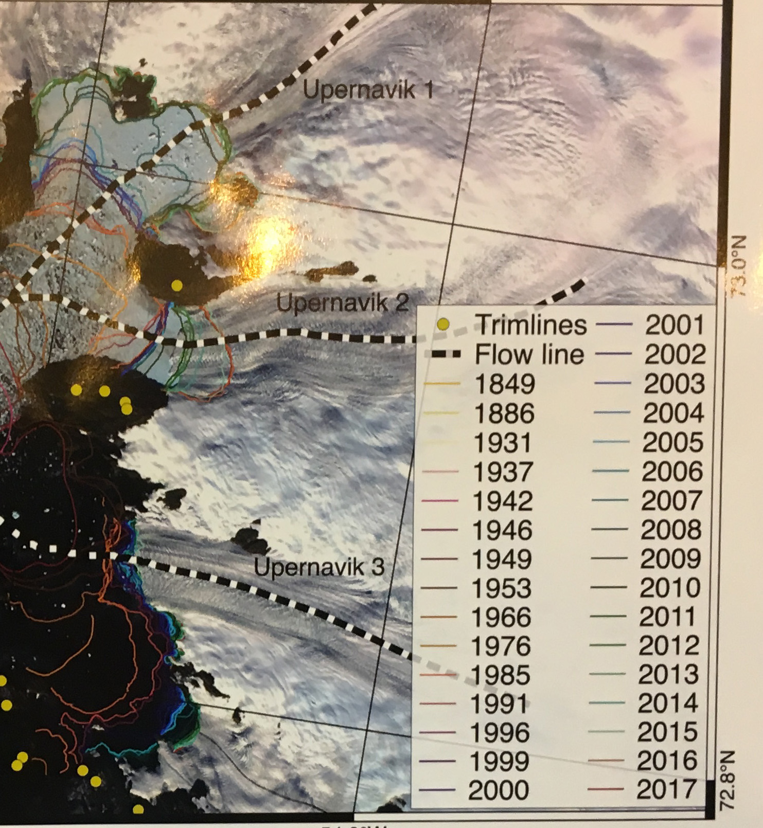
Konstanz Haubner, with a team from GEUS in Denmark provided a model simulating velocity and ice thickness change at Upernavik Glacier, Greenland from 1849-2017. In the image above the retreat is illustrated, separating into three separate glaciers with a more bedrock pinning points to stabilize.  They noted  a changing contribution to Upernavik’s ice mass loss from surface melt and ice dynamics in different time periods.


Glacier Retreat Generating New Islands List

Climate change has been driving the recession of glaciers and ice sheets, which in turn has been changing our maps.  One notable category of physical geographic features indicative of the change due to the retreat is the formation of new islands.  Below is a list of new islands that this blog has identified and reported.  This is not a comprehensive list of all islands that have been formed.  

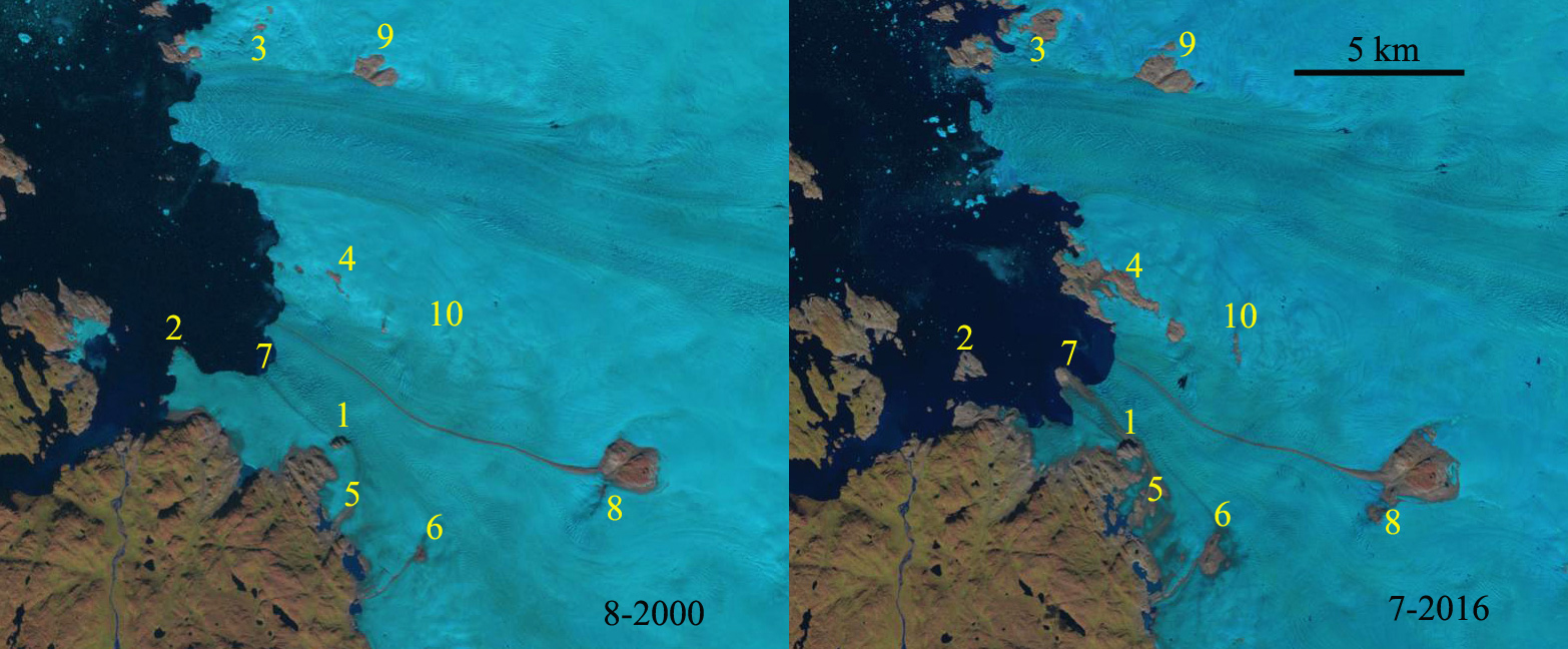
Upernavik Glacier, Greenland in Landsat images from August 2000 and August 2016.  Each Point is at the same location in both image, and the changes are noted in the discussion below.  The same locations are also identified in the July 2001 and Aug. 2016 image below. 

Kong OscarGreenland: Island A forms with B and C on the verge.

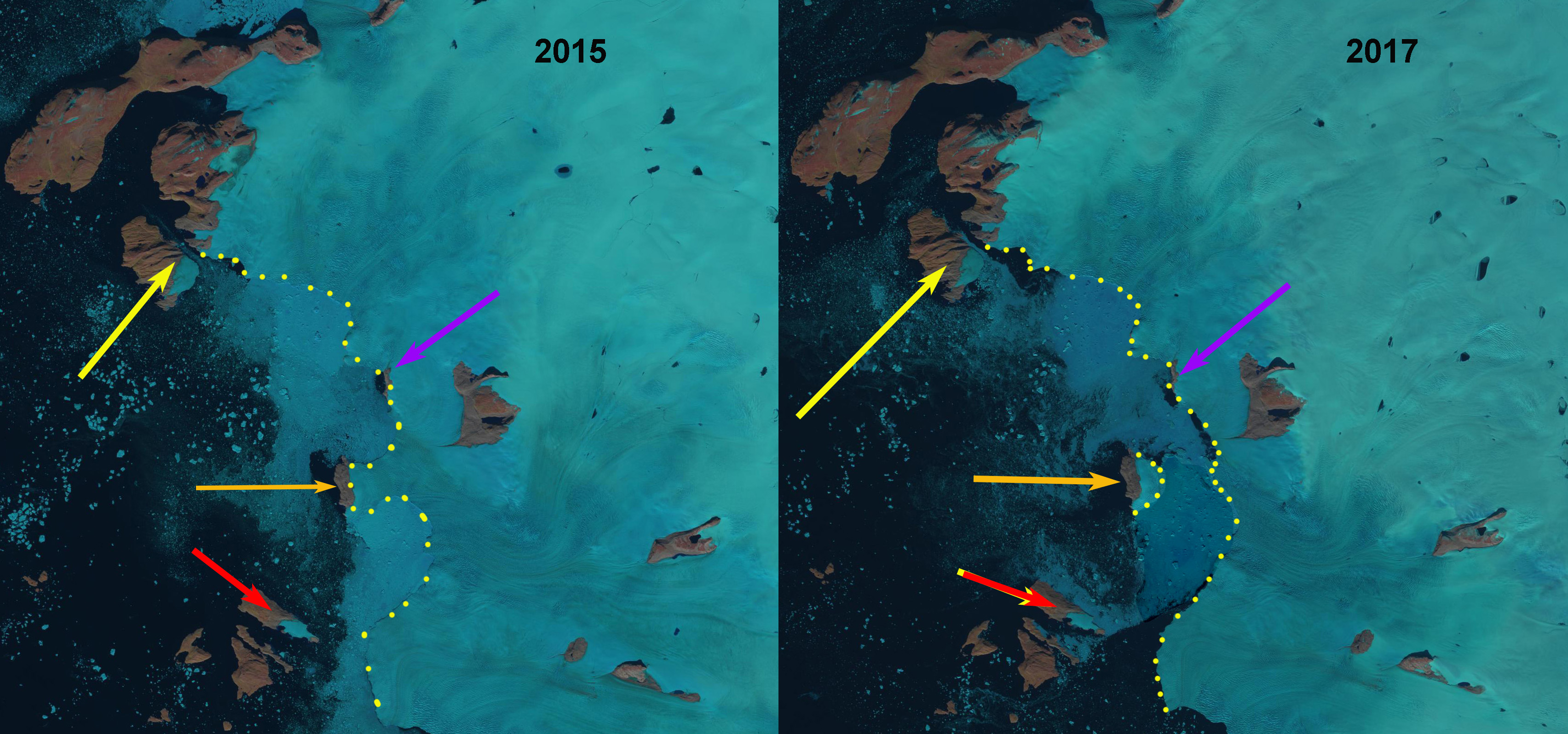
Steenstrup Glacier, Greenland front in 2015 and 2017 illustrating location with respect to the new islands at: Red Head-red arrow, Tugtuligssup Sarqardlerssuua at yellow arrow , and the 2017 new island at orange arrow.  Yellow dots indicate icefront and purple arrow another future island to be released from the glacier.  

corontation-compare-copy

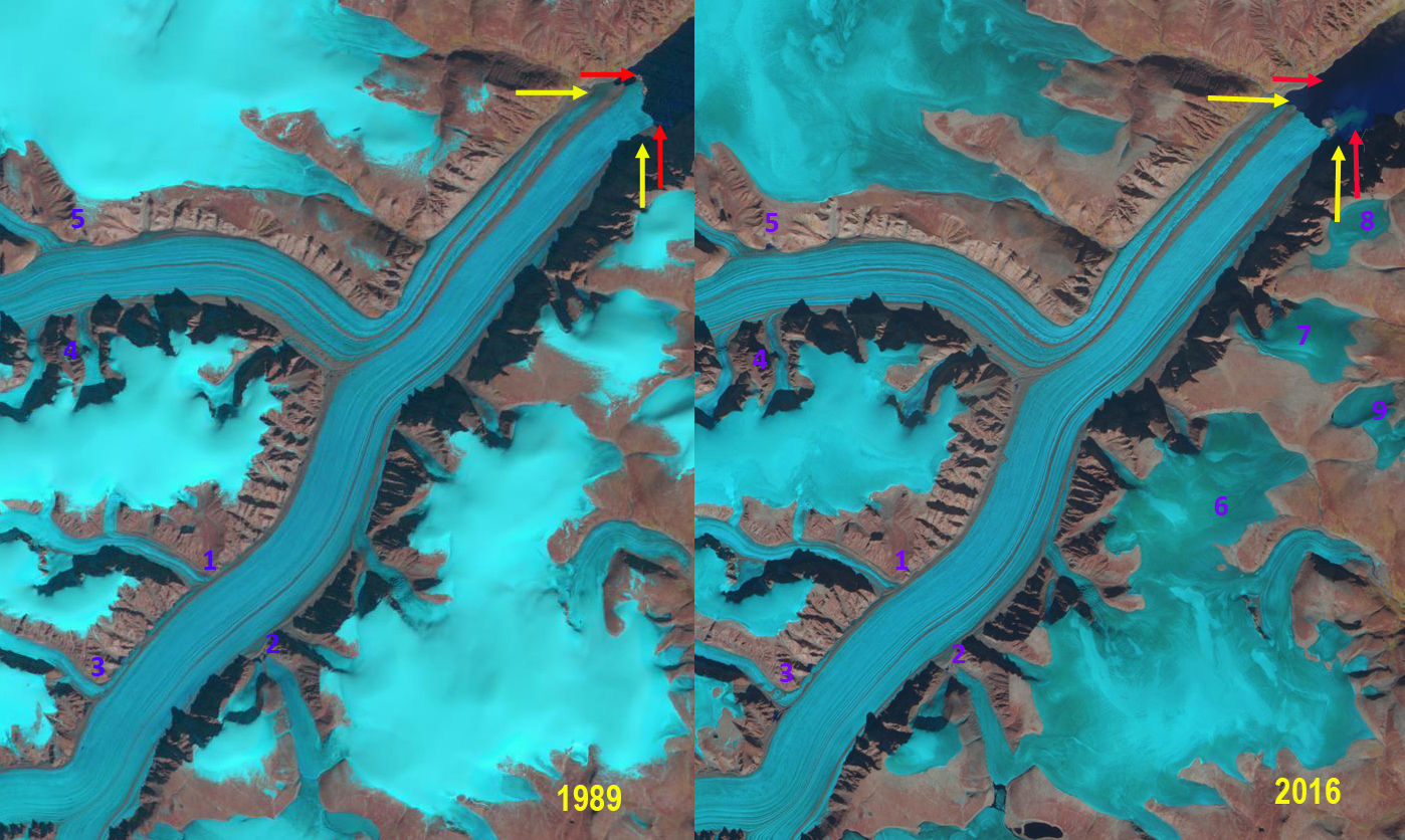
Coronation Glacier, Canada: A Landsat image from 1989 and a Sentinel 2 image from 2016 illustrate the retreat of Coronation Glacier.  Red arrows indicate the 1989 terminus and yellow arrows the 2016 terminus location.  Purple numbers 1-5 indicate locations of tributary retreat or thinning. Purple numbers 6-9 are icecaps that did not retain snowcover in 2016. 

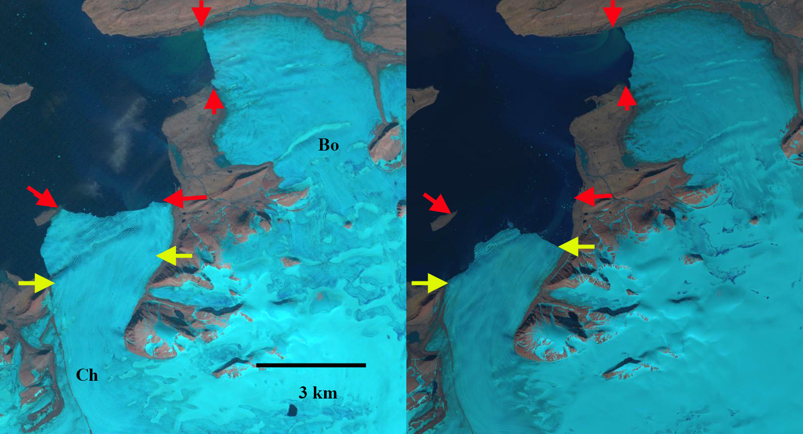
Chernysheva Glacier and Borozova, Novaya Zemlya comparison in 1990 and 2015 Landsat images. Red arrows indicates 1990 terminus and yellow arrow 2015 terminus position. Island has formed at the 1990 terminus position of Chernysheva.

Tasija and Krayniy GlacierNovaya Zemlya: Tasija Glacier (T) and Krayniy Glacier (Ky) compared in 1990 and 2015 Landsat images.  Red arrows indicate 1990 terminus positions, yellow arrows 2015 terminus positions and purple arrows upglacier thinning. A new island formed upper right red arrow.

Nizkiy Glacier, Novaya ZemlyaNizky Glacier (N) and Glasnova Glacier (G) compared in 1990 and 2015 Landsat images.  Red arrows indicate 1990 terminus positions, yellow arrows 2015 terminus positions and purple arrows upglacier thinning.  An island has formed at the second red arrow from the bottom.

Krivosheina GlacierNovaya Zemlya:  Krivosheina Glacier compared in 1990 and 2015 Landsat images.  Red arrows indicate 1990 terminus positions, yellow arrows 2015 terminus positions and purple arrows upglacier thinning.  Point A indicates a new island that has formed.

Vilkitskogo GlacierNovaya ZemlyaVilkitskogo South Glacier (Vs) and Vilkitskogo North Glacier (Vn) compared in 1990 and 2015 Landsat images.  Red arrows indicate 1990 terminus positions, yellow arrows 2015 terminus positions and purple arrows upglacier thinning.


Vasilievebreen, Svalbard: retreat from 1990-2017 has led to the creation of one island at the pink arrow, while the island at the orange arrow has eroded and an island at the white arrow is on the verge of being released by the glacier.  

Samarinbreen, Svalbard: Landsat imagery from 1990-2014 illustrates that the retreat of the glacier has been 2.1 km including the formation of an island.

Record High Mont Blanc, France Glacier August Snow Lines 2017

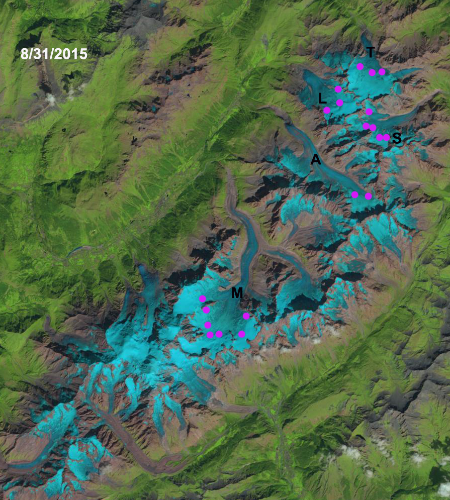
Landsat image of the transient snow line on Mont Blanc Glaciers, France on 8/19/2017.  The average snow line (Purple dots) is at 3100 m.  Glaciers on Mer de Glace (M), Argentiere (A), Tour Glacier (L), Trient Glacier (T) and Saleina Glacier (S). 

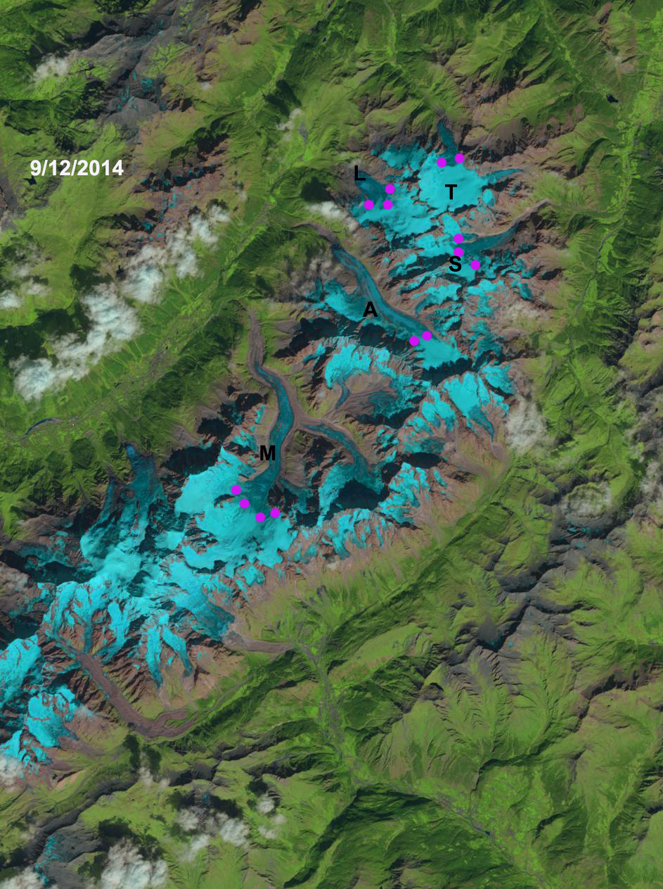
This has been a warmer summer in the Alps with reports emerging of various summer ski areas that take advantage of glaciers closing early or adding snow guns to stay open, Molltal Glacier, Les2Alpes,, Stelvio Glacier  Here we compare in Landsat images the transient snow line on five Mont Blanc glaciers from 1985, 1988, 2003, 2014, 2015 and 2017.  The transient snow line is indicated with purple dots in each image.  A comparison of the transient snow line on Mont Blanc glaciers on 8/19/2017 to other years indicates it is already higher than all other years examined, but a month remains in the melt season. 

Rabatel et al (2013)  examined the equilibrium line altitude (ELA) of glaciers in the region from 1984-2010.  The ELA is the snowline at the end of the summer melt season.  The transient snow line is simply the snow line altitude on a specific day during the melt season. Rabatel et al (2013) found the average snow line of 3000 m on Trient Glacier, 2900 m on Tour Glacier, 2800 m on Argentiere Glacier and 2975 m on Saleina Glacier.  They also observed the maximum snowline occurred in the western Alps in 2003 with an average of ~3250 m, this average is higher than for just the Mont Blanc glaciers. 

On August 11, 1985 the snow line averages 2800 m on the five glaciers.  In 1988 on Sept. 12 the snowline averages 2900 m.  On August 5, 2003 the average snow line is at 3025 m.  On Sept. 12 2014 the average snow line is at 2850 m.  On Aug. 31, 2015 the average snow line is at 3050 m.  On Aug. 19th 2017 the average snow line is at 3100 m.  This is the highest observed August snow line on Mont Blanc. With several weeks to go the snow line is competition with 2003 for the highest snow lines on Mont Blanc glaciers in the last 50 years by the end of the melt season. 

Six and Vincent (2014) noted for Argentiere Glacier that for each 1 C rise in temperature the ELA rises 50 m.  The higher snow line in 2017 indicates a year of significant negative mass balance, which will further enhance retreat of the the Mont Blanc glaciers, such as Mer de Glace and Tour Glacier. 

Landsat image of the transient snow line on Mont Blanc Glaciers, France on 8/5/2003.  The average snow line (Purple dots) is at 3000 m.  Glaciers on Mer de Glace (M), Argentiere (A), Tour Glacier (L), Trient Glacier (T) and Saleina Glacier (S).

Landsat image of the transient snow line on Mont Blanc Glaciers, France on 8/11/1985.  The average snow line (Purple dots) is at 2800 m.  Glaciers on Mer de Glace (M), Argentiere (A), Tour Glacier (L), Trient Glacier (T) and Saleina Glacier (S).


Landsat image of the transient snow line on Mont Blanc Glaciers, France on 9/12/1988.  The average snow line (Purple dots) is at 2900 m.  Glaciers on Mer de Glace (M), Argentiere (A), Tour Glacier (L), Trient Glacier (T) and Saleina Glacier (S). 

Landsat image of the transient snow line on Mont Blanc Glaciers, France on 9/12/2014.  The average snow line (Purple dots) is at 2850 m.  Glaciers on Mer de Glace (M), Argentiere (A), Tour Glacier (L), Trient Glacier (T) and Saleina Glacier (S). 

Landsat image of the transient snow line on Mont Blanc Glaciers, France on 8/31/2015.  The average snow line (Purple dots) is at 3050 m.  Glaciers on Mer de Glace (M), Argentiere (A), Tour Glacier (L), Trient Glacier (T) and Saleina Glacier (S). 

Mensu Glacier, Siberia Russia Retreat 1994-2016

Mensu Glacier, Russia in comparison of 1994 and 2016 Landsat images.  Red arrow is the 1994 terminus, yellow arrow 2016 terminus, purple arrow a tributary and purple dots the snowline. 

Mensu Glacier (Lednik Mensu) drains northeast from Gora Belukha in the Russian Altai.  The glacier drains into the Ob River and then the Arctic Ocean.  This glacier has not been the focus of detailed research to date. Khromova et al (2014) report that at the end of the century the glacier degradation in Russian mountain ranges strengthened including glacier area loss of 13% in the Tien Shan, 19% in the Altai and 22.3% in the Polar Urals.  The icecap draining west from Gora Belukha was cored to look at longer term climate records (Fujita et al 2004).  The core at 4500 m is high enough so that significant melt events affecting the record were rare. Shahgedanova et al (2010) noted that the retreat has largely been driven by summer warming. 

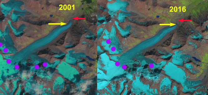
In 1994 the glacier terminates at the red arrow at 2150 m.  The glacier has an icefall from 3200 m to 2700 m that generates annual ogives, note Google Earth image below. The snowline in the 1994 Landsat  image averages 3000 m.  There is a tributary joining the main glacier at the purple arrow.  A neighboring glacier terminates in a proglacial lake at the orange arrow.  By 2001 the glacier has retreated and the snowline is at 3100 m. By 2016 the glacier terminates at 2200 m and has retreated 600  m to the yellow arrow.  The tributary at the purple arrow has separated from the main glacier.  This illustrates substantial glacier thinning  6 km above the terminus. The glacier at the orange arrow  no longer reaches the proglacial lake. In August 2016 below the snowline is at 3100 m in September 2016 the snowline has descended to 2800 m.  The lowest 800 m of the glacier has few crevasses, appears stagnant and will be lost to retreat.

Retreat is similar to the nearby Potanin Glacier, Mongolia. 

Mensu Glacier, Russia in comparison of 2001 and 2016 Landsat images.  Red arrow is the 1994 terminus, yellow arrow 2016 terminus, purple arrow a tributary and purple dots the snowline. 

Google Earth image indicating the snowline at the top of the icefall and the ogives beginning at the bottom near the orange arrow.


Terminus of Mensu Glacier in 2013 note lack of crevassing.

Llewellyn Glacier, BC Proglacial Lake Merging From Retreat

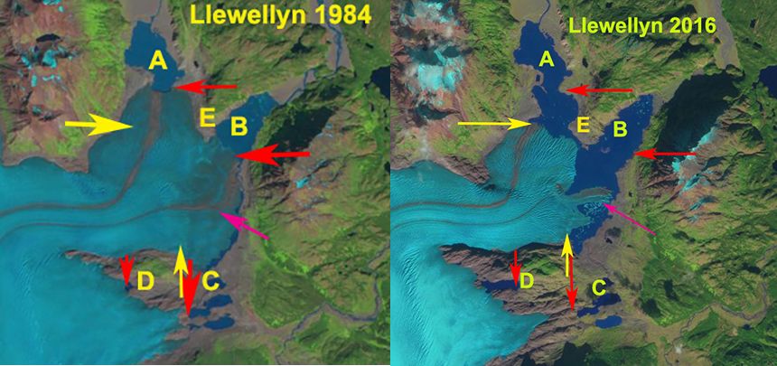
Llewellyn Glacier comparison in 1984 Landsat and 2016 Sentinel images.  Red arrows the 1984 terminus locations for proglacial lakes A-D, yellow arrows the 2016 terminus locations for A and B. Point E was the peninsula separating proglacial lakes A and B, which are now joined due to glacier retreat. 

The second largest glacier of the Juneau Icefield is the Llewellyn Glacier which is in British Columbia. The Juneau Icefield Research Program has a research camp, C-26 on this glacier and it is the typical exit route from the icefield at the end of the field season.  Here we examine changes in the terminus from 1984-2016 as a result of higher snowlines indicative of an expanded ablation zone and negative mass balance. 

I first visited the glacier in 1981 and I was also on the icefield in 1984 when the Landsat image was acquired that is used as the start point for comparison. In 1984 the glacier had several termini ending in proglacial lakes A-D. We exited the glacier on the west side of proglacial lake A in 1984 onto a proglacial outwash plain referred to as the ball bearing highway.   At Point B the terminus ended in a deeper wider proglacial lake than Lake A. At Point C and D the glacier ended in a series of small lakes.  Point E is the peninsula separating proglacial lake A and B in 1984. Proglacial Lake B had a surface water level 10-15 m higher than Lake A in 1984. In 2011 the glacier still reached Point E  separating the two lakes, which still had different water levels. In 2013 the gap first opened between the two lakes, and the water level fell in Lake B. In the summer of 2016 and spring of 2017 the gap has persisted and widened to  150 m.  From 1984 to 2016 the terminus in Lake A has retreated 1300 m, the terminus at Lake B 2100 m, terminus at Point C 800 m and terminus at Point D 1100 m. The narrow tongue of ice at the pink arrow will not survive long. The crevasse pattern suggests the glacier has another 1.5- 2 km to retreat before lake development will cease. 

The snowline during the 1998-2013 period averaged 1900 m too high for an equilibrium balance.  In a sequence of images from 2013 illustrates the rise is snowline from  1450 m on June 21,  to 1780 m on August 1 and  1810 m on Sept. 2.   The persistently higher snowlines since 1990 have led substantial thinning, Melkonian et al. (2013) note thinning of more than 1 m per year at the terminus diminishing to little change above 1500 m from 2000-2009. This will drive continued retreat, supplemented by calving into the still growing proglacial Lake at Point A and B.  The retreat of this glacier follows that of other glaciers of the Juneau Icefield including nearby Tulsequah Glacier, noted by Pelto et al (2013) and Pelto (2016) .

[ngg_images source=”recent_images” display_type=”photocrati-nextgen_basic_slideshow” gallery_width=”600″ gallery_height=”400″ cycle_effect=”fade” cycle_interval=”5″ show_thumbnail_link=”1″ thumbnail_link_text=”[Show thumbnails]” order_by=”sortorder” order_direction=”ASC” returns=”included” maximum_entity_count=”4″]

A River Runs 40 km Across the Greenland Ice Sheet

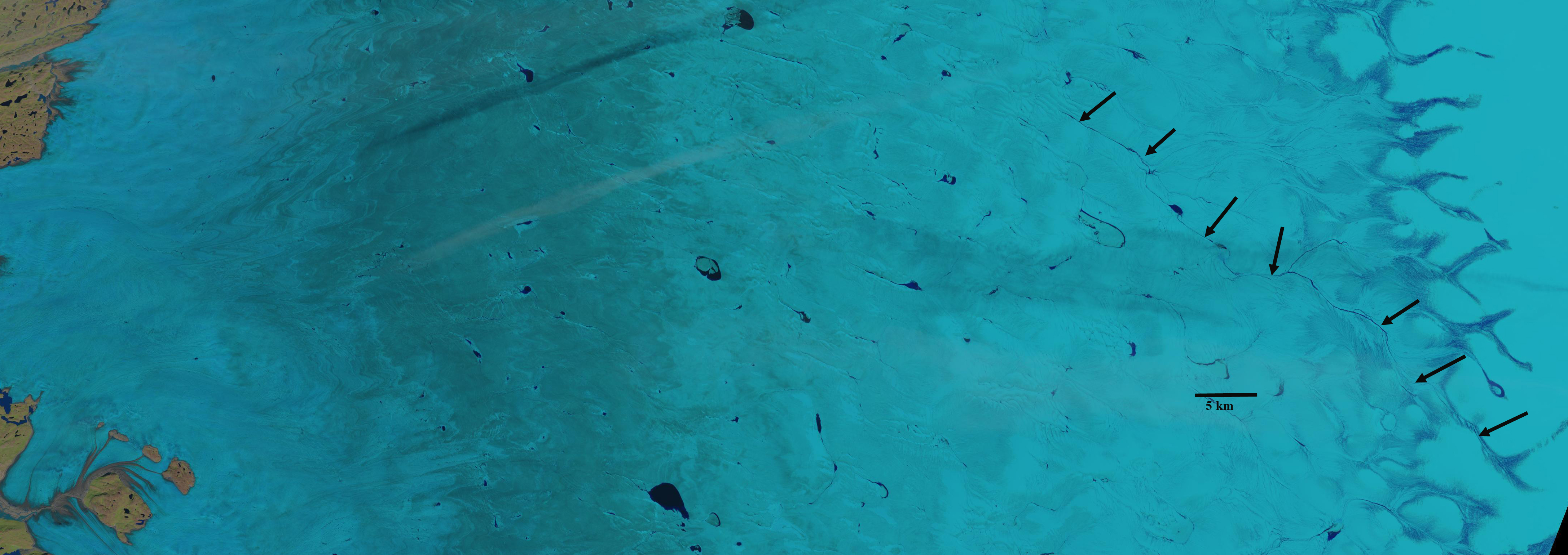
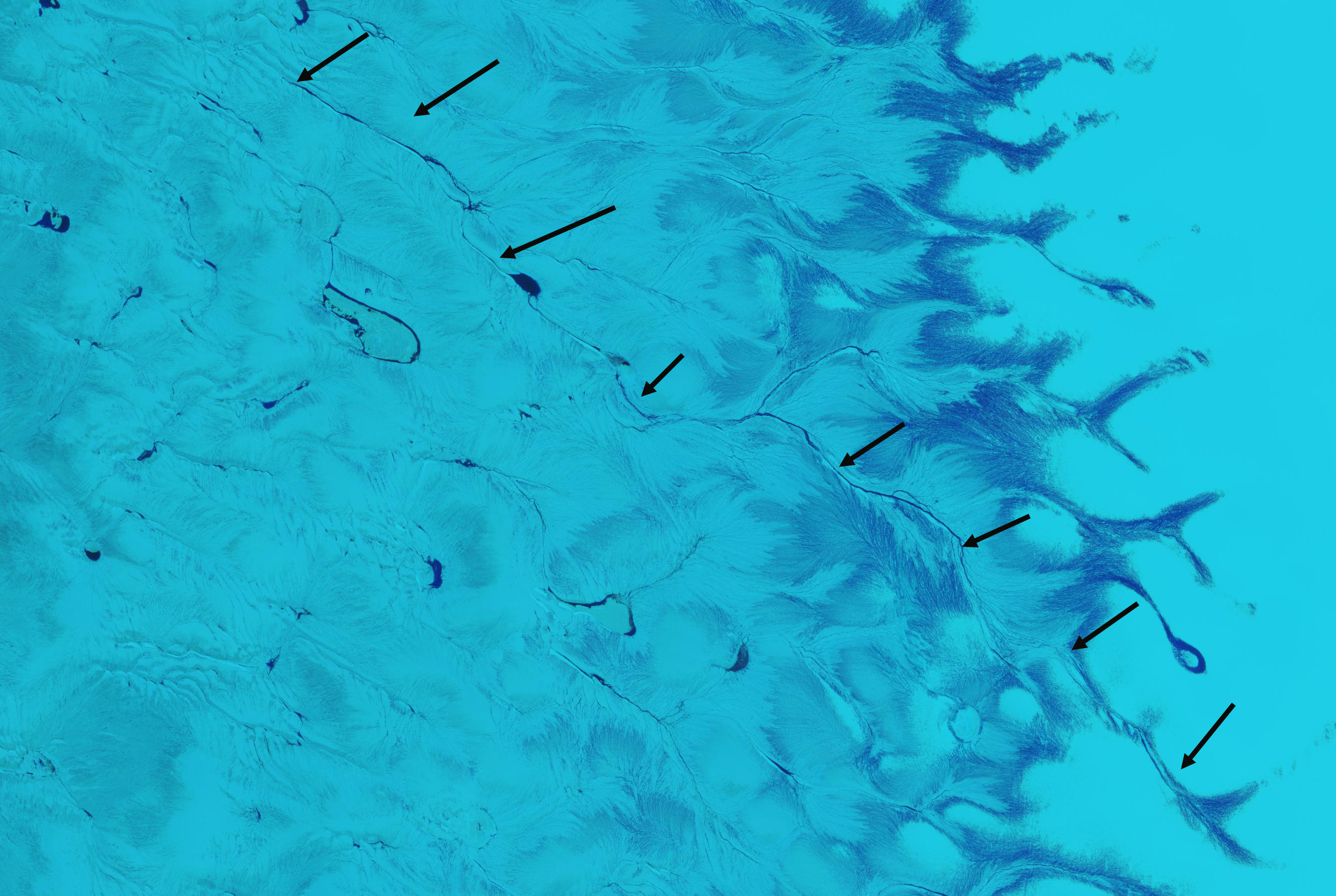
Supraglacial stream, on July 26, 2016 Landsat image, stretching 40 km across the ice sheet from the transient snowline, which marks the boundary between the percolation zone and the wet snow zone,  west toward the ice sheet margin, note black arrows.  

The Greenland Ice Sheet has experienced a significant increase in surface melt.  This is due both to warmer temperatures and enhanced melt due to a reduction in reflectivity-albedo. The expansion in melt area, duration and intensity (NSIDC, 2015)  has also generated large volume of meltwater transported via supraglacial streams.  Recent work by Tedesco et al (2016) and Kintisch et al (2017) illustrate three key reasons for the albedo change in the melt zone.

1) Upon melting and refreezing, ice crystals lose their branched shape, grow larger and rounder, which reduces the reflectivity of the snow by as much as 10%.

2) Satellite data show that the margins of the ice sheet have darkened by as much as 5% per decade since 2001. Dust trapped over the centuries has become concentrated at the melting edge of the ice sheet.

3)   The combination of algae and bacteria with dust generates a sludge—known as cryoconite. This dark material gathers in depressions decreasing albedo. Black and Bloom is a project focused on how dark particles (black) and microbial processes (bloom) darken and accelerate the melting of the Greenland Ice Sheet

Tedesco et al (2016) noted the negative trend in albedo is confined to the regions of the ice sheet that experience summer melting. They also observed no trend during the 1981–1996 period. Their analysis indicates the albedo decrease is due to the combined effects of increased air temperatures, which enhances melt promoting growth in snow grain size and the expansion of bare ice areas, and to increasing concentration of dark impurities on ice surfaces. Kintisch et al (2017) noted the same mechanisms with warmer summers also enhancing microbes and algae growth on the wetter surface of the ice, producing more cryocontie, that reduces albedo absorbing more solar energy. Cryoconite is more spatially limited than the other mechanisms. They also observed that soot and dust that blow in from lower latitudes and darken the ice are also increasing.

The darker surface enhances melt which generates more meltwater largely drained in the melt zone by supraglacial streams. Smith et al (2015) documented the surface drainage in the ablation zone of the southwest GIS. They focused on documenting the distribution of over 500 high order stream channel networks in a 6812 square kilometer region, inland from Kangerlussuaq.  All of the stream networks terminated in moulins before the ice sheet edge (NASA, 2015).  This indicates that moulins are common, important and sparse.

Poinar et al (2015) observe the longest streams in the 30-50 km range. Here we examine two streams one in detail using Google Earth that is 30 km long and a 40 km long surface stream in 2016 observed in Sentinel 2 and Landsat images. That the surface rivers can travel this distance across the surface before draining via a moulin indicates that the glacier is not structurally like Swiss cheese (Pelto, 2015).  The Google Earth detailed view illustrates both the darker surface, the maturity and hydrologic efficiency of the thermally incised meltwater streams.

The stream observed in Google Earth in its mid-reach has an average of 15 m in width.  The slope of the ice sheet is 1/120 in this region, with the river beginning at 1320 m and ending at 1070 m.  Gleason et al (2016) examined numerous supraglacial streams and noted that supraglacial streams with a width of 15-20 m and slopes of 1/100 to 1/200 had a depth of 1.5-2.0 m and velocity of ~0.5 m/sec.  This suggests the stream here has a discharge  of 7-10 cubic meters per second. The darkness of the ice surface indicating a low albedo is also apparent.  The ice is not nearly as dark when standing directly on it as it is in the macro-scale.

[ngg_images source=”galleries” container_ids=”52″ display_type=”photocrati-nextgen_basic_imagebrowser” ajax_pagination=”1″ template=”/nas/wp/www/sites/blogsorg/wp-content/plugins/nextgen-gallery/products/photocrati_nextgen/modules/ngglegacy/view/imagebrowser-caption.php” order_by=”sortorder” order_direction=”ASC” returns=”included” maximum_entity_count=”500″]

The second stream is seen in a Sentinel  image from July 15 and a Landsat image from July 26. The black arrow indicate the stream that is 40 km long.  The stream extends from 110 km from the edge of the ice sheet to within 75 km. The stream begins near the transient snowline at 1650 m and ends near 1400 m, creating a slushy valley above the local percolation zone. The stream in early July flows through the wet snow zone. By the end of the July the lower section of the stream becomes a bare ice region, the upper remains in the  wet snow zone.

Supraglacial stream in mid-July Sentinel images stretching 40 km across the ice sheet from the transient snowline west toward the ice sheet margin. 


State of Alpine Glaciers in 2016-Negative for 37th Consecutive Year

Figure 1. Global Alpine glacier annual mass balance record of reference glaciers submitted to the World Glacier Monitoring Service.

Each year I write the section of the BAMS State of the Climate on Alpine Glaciers.  What follows is the initial draft of that with a couple of added images and an added paragraph.

The World Glacier Monitoring Service (WGMS) record of mass balance and terminus behavior (WGMS, 2015) provides a global index for alpine glacier behavior.  Globally in 2015 mass balance was -1177 mm for the 40 long term reference glaciers and -1130 mm for all 133 monitored glaciers.  Preliminary data reported to the WGMS from Austria, Canada, Chile, China, France, Italy, Kazakhstan, Kyrgyzstan, Norway, Russia, Switzerland and United States indicate that 2016 will be the 37th consecutive year of without positive annual balances with a mean loss of -852 mm for reporting reference glaciers.

Alpine glacier mass balance is the most accurate indicator of glacier response to climate and along with the worldwide retreat of alpine glaciers is one of the clearest signals of ongoing climate change (Zemp et al., 2015).  The ongoing global glacier retreat is currently affecting human society by raising sea-level rise, changing seasonal stream runoff, and increasing geohazards (Bliss et al, 2014; Marzeion et al, 2014).  Glacier mass balance is the difference between accumulation and ablation.  The retreat is a reflection of strongly negative mass balances over the last 30 years (Zemp et al., 2015).  Glaciological and geodetic observations, 5200 since 1850, show that the rates of early 21st-century mass loss are without precedent on a global scale, at least for the time period observed and probably also for recorded history (Zemp et al, 2015). Marzeion et al (2014) indicate that most of the recent mass loss, 1991-2010 is due to anthropogenic forcing.
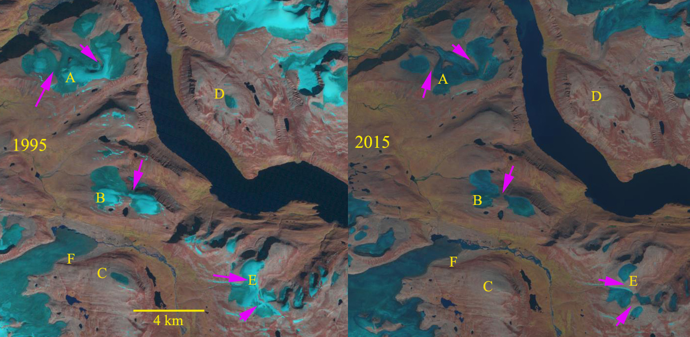
The cumulative mass balance loss from 1980-2015 is -18.8 m water equivalent (w.e.), the equivalent of cutting a 21 m thick slice off the top of the average glacier (Figure 2).  The trend is remarkably consistent from region to region (WGMS, 2015).  WGMS mass balance based on 40 reference glaciers with a minimum of 30 years of record is not appreciably different from that of all glaciers at -18.3 m w.e.  The decadal mean annual mass balance was -228 mm in the 1980’s, -443 mm in the 1990’s, 676 mm for 2000’s and – 876 mm for 2010-2016.  The declining mass balance trend during a period of retreat indicates alpine glaciers are not approaching equilibrium and retreat will continue to be the dominant terminus response. The recent rapid retreat and prolonged negative balances has led to some glaciers disappearing and others fragmenting (Figure 2)(Pelto, 2010; Lynch et al, 2016).

Below is a sequence of images from measuring mass balance in 2016 in Western North America from Washington, Alaska and British Columbia.  From tents to huts, snowpits to probing, crevasses to GPR teams around the world are assessing glacier mass balance in all conditions.

[ngg_images source=”galleries” container_ids=”7″ display_type=”photocrati-nextgen_basic_imagebrowser” ajax_pagination=”1″ template=”/nas/wp/www/sites/blogsorg/wp-content/plugins/nextgen-gallery/products/photocrati_nextgen/modules/ngglegacy/view/imagebrowser-caption.php” order_by=”sortorder” order_direction=”ASC” returns=”included” maximum_entity_count=”500″]

Much of Europe experienced record or near record warmth in 2016, thus contributing to the negative mass balance of glaciers on this continent. In the European Alps, annual mass balance has been reported for 12 glaciers from Austria, France, Italy and Switzerland. All had negative annual balances with a mean of -1050 mm w.e.  This continues the pattern of substantial negative balances in the Alps continues to lead to terminus retreat.  In 2015, in Switzerland 99 glaciers were observed, 92 retreated, 3 were stable and 4 advanced.  In 2015, Austria observed 93 glaciers; 89 retreated, 2 were stable and 2 advanced, the average retreat rate was 22 m.

In Norway, terminus fluctuation data from 28 glaciers with ongoing assessment, indicates that from 2011-15 26 retreated, 1 advanced and 1 was stable.  The average terminus change was -12.5 m (Kjøllmoen, 2016).  Mass balance surveys with completed results are available for seven glaciers; six of the seven had negative mass balances with an average loss of -380 mm w.e.

In western North America data has been submitted from 14 glaciers in Alaska and Washington in the United States, and British Columbia in Canada.  All 14 glaciers reported negative mass balances with a mean loss of -1075 mm w.e.  The winter of and spring of 2016 were exceptionally warm across the region, while ablation conditions were close to average.

In the high mountains of central Asia five glaciers reported data from Kazakhstan, Kyrgyzstan and Russia.  Four of five were negative with a mean of -360 mm w.e.  Maurer et al (2016) noted that mean mass balance in the eastern was significantly negative for all types of glaciers in the Eastern Himalaya from 1974-2006.

Figure 2. Landsat images from 1995 and 2015 of glaciers in the Clephane Bay Region, Baffin island.  The pink arrows indicate locations of fragmentation.  Glaciers at Point C and D have disappeared.


Cook Ice Cap Outlet Glacier Retreat Lake Fromation, Kerguelen 2001-17


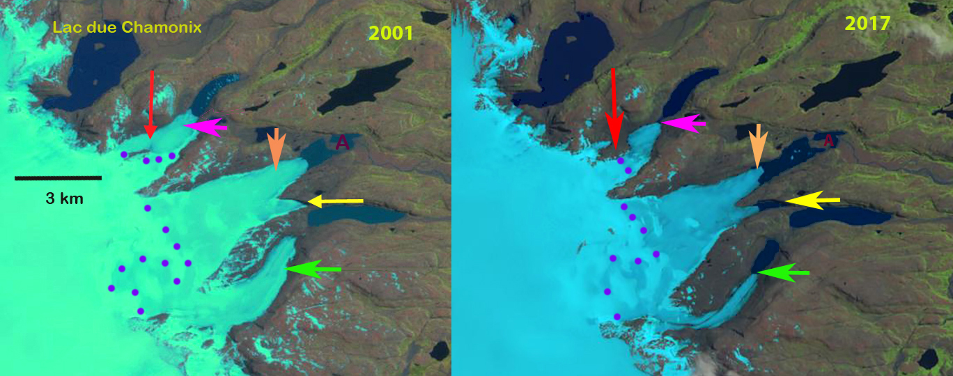
Comparison of eastern outlet glaciers of the Cook Ice Cap in 2001 and 2017 Landsat images.  Red arrow indicates a location of tributary separation. Pink arrow the 2017 terminus location of the northernmost glacier. Orange arrow the 2017 terminus location of the middle glacier.  Yellow arrow tip the 2001 terminus position of glacier ending in newly formed lake.  Green arrow the southernmost glacier 2017 terminus location. 

On the east side of the Cook Ice Cap on Kerguelen Island a series of outlet glaciers have retreated expanding and forming a new group of lakes.  Here we examine the changes from 2001-2017 along using Landsat imagery. Retreat of glacier in the region was examined by Berthier et al (2009) and is exemplified by the retreat of Ampere Glacier.  Verfaillie et al (2016) examined the surface mass balance using MODIS data, field data, and models.  They identified that accelerating glacier wastage on Kerguelen Island is due to reduced net accumulation and resulting rise in the transient snowline since the 1970s, when a significant warming began.

In 2001 at the red arrow is where the north tributary of a glacier ending in the northern most lake joins the main glacier.  In the second lake is a peninsula, marked with point A that the glacier terminus is 1 km from. The next two glaciers terminating at the yellow arrow and beyond the green arrow do not have lakes at their termini.  By 2014 the northern tributary has lost its connection with the main glacier terminating in the lake. The distance from the island for the middle glacier has increased.  A lake is forming at the yellow arrow. For the third glacier a lake has formed at the green arrow. In 2017 the northern glacier has retreated to the pink arrow a distance of  750 m and is no longer terminating in the lake. The terminus at the orange arrow has retreated  main terminus has retreated 900 m, expanding the lake it terminates in.   The glacier at the yellow arrow has retreated into a new lake basin, with a retreat of 850 m since 2001. The terminus is thin and in the Google Earth image indicates some substantial thin icebergs have separated from the glacier. The green arrow marks the 2017 terminus of the southern most lake. This glacier has retreated 950 m leading to the continued expansion of a new lake.  In just a decade we see the formation of two new lakes and the expansion of two others at the terminus of the eastern outlet glaciers of Cook Ice Cap, rapid landscape change driven by climate change.

2014 Landsat image of the eastern outlet glaciers of Cook Ice Cap.Red arrow indicates a location of tributary separation. Pink arrow the 2017 terminus location of the northernmost glacier. Orange arrow the 2017 terminus location of the middle glacier.  Yellow arrow tip the 2001 terminus position of glacier ending in newly formed lake.  Green arrow the southernmost glacier 2017 terminus location. 

Terminus of three outlet glaciers from left to right the green arrow, yellow arrow and orange arrow terminus glacier on the Landsat images.  The green arrows indicate places where the terminus or icebergs illustrates how thin the glacier ice is. 

Recent Climate Change Impacts on Mountain Glaciers – Volume

fig10-1

Landsat Image of glaciers examined in the Himalaya Range: Chapter 10 that straddles a portion of Sikkim, Nepal and Tibet, China. Notice the number that end in expanding proglacial lakes. 

This January a book I authored has been published by Wiley. The goal of this volume is to tell the story, glacier by glacier, of response to climate change from 1984-2015. Of the 165 glaciers examined in 10 different alpine regions, 162 have retreated significantly. It is evident that the changes are significant, not happening at a “glacial” pace, and are profoundly affecting alpine regions. There is a consistent result that reverberates from mountain range to mountain range, which emphasizes that although regional glacier and climate feedbacks differ, global changes are driving the response. This book considers ten different glaciated regions around the individual glaciers, and offers a different tune to the same chorus of glacier volume loss in the face of climate change. There are 107 side by side Landsat image comparisons illustrating glacier response.  Several examples are below: in each image red arrows indicate terminus positions from the 1985-1990 period and yellow arrows terminus positions for the 2013-2015 period, and purple arrows upglacier thinning.

[ngg_images source=”galleries” container_ids=”17″ display_type=”photocrati-nextgen_basic_imagebrowser” ajax_pagination=”1″ template=”/nas/wp/www/sites/blogsorg/wp-content/plugins/nextgen-gallery/products/photocrati_nextgen/modules/ngglegacy/view/imagebrowser-caption.php” order_by=”sortorder” order_direction=”ASC” returns=”included” maximum_entity_count=”500″]

There are chapters on: Alaska, Patagonia, Svalbard, South Georgia, New Zealand, Alps, British Columbia, Washington, Himalaya, and Novaya Zemlya. If you are a frequent reader of this blog you will recognize many of the locations. This updates each glacier to the same time frame. The book features 100 side by side Landsat image pairs illustrated using the same methods to illustrate change of each glacier. The combined efforts of the USGS and NASA in obtaining and making available these images is critical to examining glacier response to climate change. The World Glacier Monitoring Service inventory of field observations of terminus and mass balance on alpine glaciers is the another vital resource.  The key indicators that glaciers have been and are being significantly impacted by climate change are the global mass balance losses for 35 consecutive years documented by the WGMS.  The unprecendented global retreat that is increasing even after significant retreat has occurred in the last few decades (Zemp et al, 2015).  Last, the decline in area covered by glaciers in every alpine region of the world that is documented by mapping inventories such as the Randolph Glacier inventory and GLIMS ( Kargel et al 2014)

fig6-2

Landsat Image of glaciers examined in the Svalbard: Hornsund Fjord Region: Chapter 6.

fig5-1

Landsat Image of glaciers examined in the South Georgia Island: Chapter 5.

fig8-9

Landsat Image of Mount Baker glaciers examined in the North Cascades, Washington:  Chapter 8.

fig11-1

Landsat Image of glaciers examined in the Southern Alps of New Zealand S: Chapter 11.


Gangotri Glacier Expanded Melt Season & Melt Area in 2016

[ngg_images source=”galleries” container_ids=”22″ display_type=”photocrati-nextgen_basic_imagebrowser” ajax_pagination=”1″ template=”/nas/wp/www/sites/blogsorg/wp-content/plugins/nextgen-gallery/products/photocrati_nextgen/modules/ngglegacy/view/imagebrowser-caption.php” order_by=”sortorder” order_direction=”ASC” returns=”included” maximum_entity_count=”500″]

Purple dots indicate the transient snowline on Gangotri Glacier in the fall and early winter of 2016. Red arrow indicates the terminus of the glacier.

The Gangotri Glacier is the largest glacier in the Bhagirathi River watershed, situated in the Uttarkashi District, India. It is one of the larger glaciers in the Himalaya, and like all of the nearby Himalayan glaciers is retreating significantly. Gangotri Glacier provides hydropower as its meltwater  passes through three hydropower plants generating 1430 MW, including the 1000 MW Tehri Dam and reservoir and Maneri Bhali I and II, see map below.  From 1968-2006 the glacier retreated 800 meters, close to 20 meters per year (Bhambri et al, 2012). The glacier continues to thin and tributary inflow decline, while terminus retreat is slowe due to the thick debris cover that heavily insulates the ice. Bhambri et al (2011) inventoried glaciers in the upper Bhagirathi basin  and found they lost 9 square kilometers in area, 3.3% to the total, from 1968 to 2006. They further noted that recession rates have increased since 1990 and that the number of glaciers increased from 82 in 1968 to 88 in 2006 due to fragmentation of glaciers. From 1968 to 2006, the debris-covered glacier area increased by ~12% in the upper Bhagirathi basin.  Bhattachaya et al (2016) expanded on this work noting that the velocity of Gangotri Glacier declined during 2006-2014  by 6.7% from 1993-2006, this suggests reduced accumulation being funneled downglacier. They also noted an increase in the rate of debris-covered area expansion on the main trunk of Gangotri Glacier from 2006-2015, which is indicative of an expanding ablation zone. Bhattachaya et al (2016)  report a retreat rate of 9 m/year 2006-2015, which is less than before, but the down-wasting in the same period 2006-2015 was higher than during 1968-2006. The study reinforced that glacier retreat is a delayed response to climate change, whereas glacier mass balance is a more direct and immediate response. This underlines the importance of mass balance studies for assessing climate change impact on glaciers,that the World Glacier Monitoring Service has emphasized. Gangotri Glacier is a summer accumulation glacier with the peak ablation period low on the glacier coinciding with peak snowfall high on the glacier during the summer monsoon.  In the post monsoon period of October and November precipitation is low and melt rates decline, Haritashya et al (2006) note a sharp decline in discharge and suspended sediment load beginning in October. . Kundu et al (2015) from Sept. 2012 to January 2013 noted that the snowline elevation varied little, with the highest elevation being 5174 m and the lowest 5080 m.

The increase in temperature has led to a tendency for snowlines to rise in the post monsoon period and remain high into the winter season on many Himalayan glaciers. In 2016 this has been the case. On October 9, 2016  a Sentinel image indicates the snowline is at 4850 m on the main trunk and on the tributary Ghanohim Glacier the snowline, while it is 4750 m on the tributaryKirti Glacier.  A Landsat image from October 13th indicates the snowline on Kirti has risen to 4800 m, and remains at 4850 on the main trunk and Ghanohim Glacier.  By November 30th a Landsat image indicates the snowline has risen to 5400 m on the main trunk and Ghanohim, the snowline is at 5800-5900 m on the glaciers in the Swachhand tributary valley, at 5600 m on Maiandi Glacier and 5700 m on the last tributary entering from the north. Note the impact of radiational shading is apparent on the main trunk with the snowline descending down the middle of the main trunk from 5400 m to 5100 m and on Kirti Glacier which is too dark to confidently discern the snowline.  Temperatures are typically cool in December, but sunshine is common. A Sentinel image from December 8th and Landsat from Dec. 9th indicate that the snowline remains approximately the same as on Nov. 30th.  The accumulation area ratio is the percentage of a glacier in the accumulation zone and is typically above 50%.  On Gangotri Glacier in December 2016 the accumulation area ratio is only 20%, indicating a large mass balance deficit.  High winter snowlines on Chutenjima Glacier, Tibet, from October, 2015 to February 2016. This tendency is also noted at Nup La-West Rongbuk Glacier, on the Nepal-China border, West Hongu Glacier, Nepal and Lhonak Glacier, Sikkim.

gangotri-glims

Gangotri Glacier and its key tributaries, with the red line being the outline of the glacier from GLIMS.

bhagirathi-150411

Hydropower in the Bhagirathi River watershed

Norrearm Fjord Glacier Retreat, Greenland

norrearm-compare

Apostelens Glacier in Norrearm Fjord Landsat comparison from 1999 to 2016. Red arrows are the 1999 terminus location, yellow arrows the 2016 terminus location and purple arrows indicate an expanding bedrock ridge.

“Apostelens” Glacier drains east from a peak of the same name into an arm of Norrearm Fjord, which in turn is part of Lindenow Fjord in southern Greenland. The glacier is a short distance north of Kangersuneq Qingordleq, where recent retreat has led to glacier separation. The glacier is soon to lose its tidewater connection as has occurred at Tasermiut Fjord to the west.  This will result in a decline in iceberg production as well.

Here we examine Landsat imagery from 1999-2016 to identify glacier change.  In 1999 the Apostelens arm of Norrearm Fjord is largely filled by the glacier which extends to within 2.5 km of Norrearm Fjord, red arrow.  The tongue contains numerous ogives formed each year due to seasonal velocity changes through an icefall.  This is evident in the Google Earth image from 2004, where 24 ogives are evident on the low slope glacier tongue, in 1999 the number is over 30. By 2013 the glacier has retreated nearly 2 km from the 1999 terminus position, red arrow. In 2012 Google Earth imagery indicates increased crevassing near the front and the loss of most ogives.  New ogive formation is also hard to distinguish.  By 2016 the glacier has retreated 2.6 km and is nearing the headward limit of the fjord arm.  The collapse of the fjord tongue and its associated ogives indicates the loss of 30 years worth of volume flux that emerged from the icefall that generated the ogives.

Greenland tidewater outlet glaciers in this region have experienced substantial retreat since 1990, Weidick et al (2012) and Howat and Eddy (2011).  Murray et al (2015) examined 199 tidewater glaciers in Greenland and noted significant retreat of 188 of them.  Apostelens Glacier was not one of these, and soon will not be a tidewater glacier to be included in the list.

norrearm-ge

Apostelens Glacier in Norrearm Fjord Google Earth comparison from 2004 and 2012. Red arrows are the 2004 terminus location, and yellow arrows the 2012 terminus location.  Note ogives in 2004 and loss of them in 2012. 

norrearm-map

Map of the Norrearm Fjord region and Apostelens Glacier, with blue arrows indicating flow. 

Hagafellsjokull, Iceland Reflects Langjokull Thinning & Retreat

hagafellsjokull-compare

Landsat comparison of the terminus of Hagafellsjökull from 2000 and 2016.  The red arrows are the 2000 terminus, the yellow arrows the 2016 terminus.  Purple arrows indicate upglacier thinning. 

Langjökull is the second largest iceap in Icalnd with an area of over 900 square kilometers. The mass balance of the icecap has been reported since 1997 and his lost over 1 m per year during this period (WGMS, 2016).  Pope et al (2010) noted that the icecap has lost an area of 3.4 ± 2.5 km2 yr-1 over the decade from 1997-2007.  Pope et al (2010) noted that the loss of ice volume confirms previously published predictions that Langjökull will likely disappear within the next 200 years if current trends continue. A key outlet of  Langjökull is  Hagafellsjökull which terminates in Hagvatn. Hagafellsjökull ended a sustained post Little Ice Age retreat in 1970.  The ensuing advance of approximately 1 km ended by 2000.  Here we examine Landsat imagery from 2000-2016 to identify recent changes in this outlet glacier.

In 2000 the glacier terminated on an island in Hagavatn, red arrow.  The east margin of the glacier featured several locations where secondary termini overflowed a low ridge on the east side of the glacier.  By 2006 the glacier had retreated 500-600 m from the island.  By 2016 the terminus had retreated across its entire width by 800-850 m, 50 m/year, yellow arrows.  A closeup view from the Iceland online map application illustrates the 2014 terminus red dots. The end of the glacier has a low slope, low velocity and is debris covered.  The western side has terminated on land during this entire period and has approximately the same retreat rate as the eastern half that still ends in the expanding lake. There is little evidence of iceberg release into the lake, which helps explain the similar retreat rate. The low slope and upglacier thinning noted at the purple arrows indicate the retreat will continue.  In 2014 the transient snowline reached near the head of the glacier at over 1100 m.  In 2000, 2006 and 2016 the snowline with several weeks left in melt season ranged from 859-950 m. The retreat is similar to that of Norðurjökull another outlet of the Langjökull and Porisjokull.
langjokull-south-outlet-ge-2010

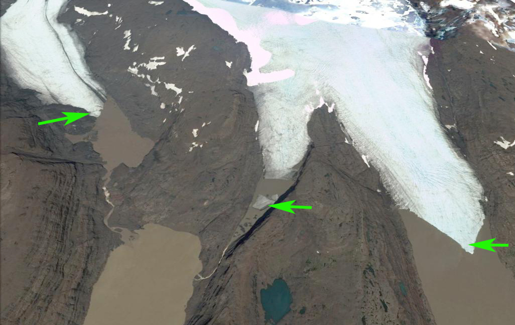
Google Earth view of the terminus of Hagafellsjökull in 2014. Red arrow is the 2000 terminus position and yellow arrow the 2014 position.

 hagafellsjokull-ismap

Online Iceland Map Viewer indicating the terminus of Hagafellsjökull in 2014, red dots.

hagafellsjokull-tsl

2006 and 2014 Landsat images of Hagafellsjökull indicating the transient snowline off the image in 2014 and at 850 m in 2006.