NORTH CASCADE GLACIER CLIMATE PROJECT 2020-37th Annual Field Program

Field season images from 2019 indicating crevasse stratigraphy, annotated by Clara Deck.

Director: Mauri S. Pelto, mspelto@nichols.edu-Nichols College

Field Artist & Scientist: Jill Pelto, pelto.jill@gmail.com

Who we are? NCGCP was founded in 1983 to identify the response of North Cascade glaciers to regional climate change, particularly changes in mass balance, glacier runoff and terminus behavior.   NCGCP is a field project that has a broader interdisciplinary scope and examines more glaciers than any other program in North America.  It does so cost effectively relying on no permanent camps, helicopter support or salaries for the director. The field season includes no days off and each day is spent completing measurements on glaciers.  The focus is on glacier mapping, mass balance measurement, terminus observations and glacier runoff monitoring.  This program monitors two of the World Glacier Monitoring Service’s reference glaciers. There are ~45 such glaciers in the world with 30 years of continuous measurements. We complete mass balance and terminus observations on Columbia, Daniels, Easton, Ice Worm, Lower Curtis, Lynch, Rainbow and Sholes Glacier with runoff measurements below Sholes and Ice Worm.

Why study glaciers in the North Cascades? Glaciers are one of the world’s best climate monitors and are a critical water resource to many populated glaciated regions. This is particularly true in the North Cascades where 700 glaciers yield 200 billion gallons of summer runoff and glaciers have lost 30 % of their area in the last century.

Field Team 2020:

Jill Pelto is an artist and scientist from New England who grew up loving winter sports and trips to the mountains. She incorporates scientific research and data into paintings and prints to communicate environmental changes. Her multi-disciplinary work weaves visual narratives that reveal the reality of human impacts on this planet, as earlier in July was illustrated on the cover of TIME. She completed both her B.A. degrees in Studio Art and Earth and Climate Sciences and her M.S. focused on studying the stability of the Antarctic Ice Sheet at the University of Maine, spending two field seasons at a remote camp in the southern Transantarctic Mountains. Jill will be joining the project for her 12th field season. She is excited about continuing to document the change in North Cascade glaciers that she has witnessed each of the last ten years — through science and art.

Mauri Pelto has directed the project since its founding in 1984, spending more than 700 nights camped out adjacent to these glaciers. He is the United States representative to the World Glacier Monitoring Service, author of the AGU blog “From a Glacier’s Perspective”, and on the Science Advisory Board for NASA’s Earth Observatory.  His primary job is Dean of Academic Affairs at Nichols College, where he has been a professor since 1989.

Cal Waichler is an environmental science major at Colby College in Maine and is from Winthrop, WA. She looks to bridge the gap between science and the public by creating impactful, accurate climate art and storytelling. This summer’s research goal is to generate building blocks to contextualize her work within two fields: glacier science and climate communication.
Mariama Dryak (she/her) is an earth scientist, science communicator/writer and an advocate for action on creating solutions to the global climate crisis. Mariama is the creator and editor of an environmental advocacy blog Let’s Do Something BIG. and the ‘we persist.’ podcast, which shares the stories of underrepresented people in the earth, ocean and environmental sciences. Mariama received her Master’s from the University of Maine in 2019 in Earth and Climate Science, during which she drew connections between inferred ocean conditions and glacier change along the Antarctic Peninsula. Mariama can most often be found chatting science, going on adventures or getting muddy whilst doing something outdoors.

Columbia Glacier terminus with the 2018 field team.

 Field Partners 2020

Victoria Jarvis and Michelle Tanz are Wilderness Stewardship Fellows who will be gathering information about the Henry M Jackson Wilderness including the glacier. They are looking to understand the Columbia Glacier and our research within the scope of the 5 qualities of wilderness character (untrammeled, undeveloped, natural, solitude and primitive rec, other). They will then be able to incorporate our long-term monitoring efforts into their wilderness character narrative– a synthesized agency document providing insight about the wilderness.

Alia Khan, Western Washington University Cryosphere Studies and Aquatic Biochemistry Lab:

The research team including grad students Molly Peek and Shannon Healy focus on environmental chemistry in the cryosphere, including black carbon and snow algae to document global change of glacier and snow melt in mountainous and polar regions.

Tom Hammond, North Cascade Conservation Council,Will be joining us for the 17th year leveraging his experience with our for understanding the ongoing impact of climate change and our stewardship on the region.
Nooksack Indian Tribe, for the 9th consecutive year we will be conducting field work aimed at providing field validation and streamflow calibration data below Sholes Glacier for the ongoing work of the tribe.

Measuring flow below Sholes Glacier

Global Glacier Change Bulletin 3 (WGMS) Reports Increasing Mass Balance Losses

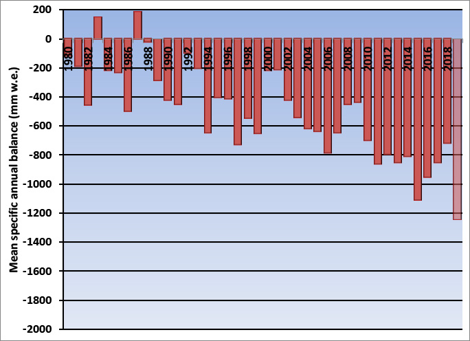
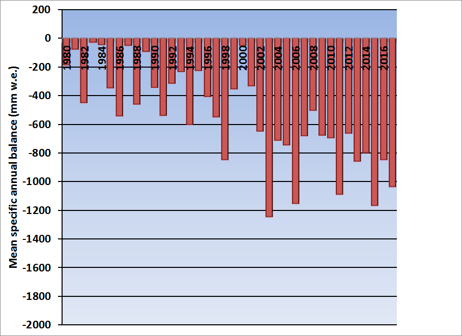
Figure 1. Regionalized mean annual mass balance of WGMS reference glaciers 1980-2018, with 2019 being a mean of reference glaciers.

Glaciers have been studied as sensitive indicators of climate for more than a century and are now experiencing a historically unprecedented decline (Zemp et al, 2015).  Glacier fluctuations in terminus position, mass balance and area are recognized as one of the most reliable indicators of climate change. This led to glacier mass balance being recognized during the International Geophysical Year (IGY) in 1957 as a key focus area for developing long term data sets and the need to establish an international data repository.

Today this data reporting system is managed by the World Glacier Monitoring Service (WGMS). WGMS annually collects standardized observations on changes in mass, volume, area and length of glaciers with time, and additionally collecting statistical information on the distribution of glaciers from inventories.  WGMS just published their third Global Glacier Change Bulletin, a comprehensive data report covering the 2015/2016 and 2016/2017 hydrologic years. I review some of that information here with updated reference glacier mass balance data from WGMS for 2018 and 2019.

The data set compiled by the World Glacier Monitoring Service has 45,840 measurements on 2540 glaciers (WGMS, 2020). Annual mass balance measurements are the most accurate indicator of short-term glacier response to climate change.  WGMS, (2020) data set has 7300 annual balance values reported from 460 glaciers, with 41 reference glaciers having 30+ year consecutive ongoing records. Annual mass balance is the change in mass of a glacier during a year resulting from the difference between net accumulation and net ablation.

The key data set is the annual balance record from the reference glacier network, these glacier have extensive continuous field monitoring programs with at least a 30 year record.  For example on Columbia Glacier, Washington I have been in the field 36 consecutive summers, over 120 days taking 4600 measurements with 63 assistants. Figure 1 above illustrates glacier mass balance for the set of global reference glaciers for the time-period 1980-2019. Global values are calculated using a single value (averaged) for each of 19 mountain regions in order to avoid a bias to well observed regions.

In the hydrological year 2016/17, observed glaciers experienced an ice loss of -550 mm, and 2017/18 of -720 mm. For 2018/19 hydrologic year a regionally averaged value will not be available until December 2020, the overall mean of all reference glaciers of -1241 mm, compared to -1183 mm in 2017/2018. This will make 2019 the 32nd consecutive year with a global alpine mass balance loss and the tenth consecutive year with a mean global mass balance below -700 mm. The simple mean mass balance of WGMS records has a slight negative bias compared to geodetic approaches, but this bias has been effectively eliminated with the regionalized approach now used by WGMS, see Figure 2 (WGMS, 2020).

Figure 2. Glaciological mass balance of all glacier, reference glaciers (mean), regional mean of reference glaciers and regionalized mean geodetic mass balances for the 1930-2017 period.  Pay particular note to the 1960-2017 period where the data records are better.  Observe the similarity in cumulative mass balance losses regardless of approach.

The decadal averaged annual mass balance was -172 mm in the 1980’s, -460 mm in the 1990’s, 500 mm for 2000’s and – 889 mm for 2010-2019.  The increasing rate of glacier mass loss, with eight out of the ten most negative mass balance years recorded after 2010, during a period of retreat indicates alpine glaciers are not approaching equilibrium and retreat will continue to be the dominant terminus response (Pelto, 2019; WGMS, 2020).  The accumulation area ratio is an indication of the expansion of the ablation areas globally, despite retreat accumulation areas are shrinking.  The decline in accumulation area extent, hence AAR has been rapid, the data in 2017/2018 yields a mean of 13%, whereas the average needed to be in balance is 56%. The low AAR in 2019 is illustrated at two reference glaciers Lemon Creek, Alaska and Alfotbreen, Norway below.

Years

Ba

AAR

1980-1989

-172

47

1990-1999

-460

44

2000-2009

-525

35

2010-2019

-889

28

Table 1 Glaciologic annual balance for each decade from the WGMS reference glacier mean of the 19 regions. The AAR is a simple mean of the reference glaciers.

Landsat images of Lemon Creek Glacier, Alaska and Alfotbreen, Norway in 2019. White dots indicate the glacier boundary on Alfotbreen, purple dots the snowline. Lemon Creek AAR=0%  Alfotbreen AAR=~15%

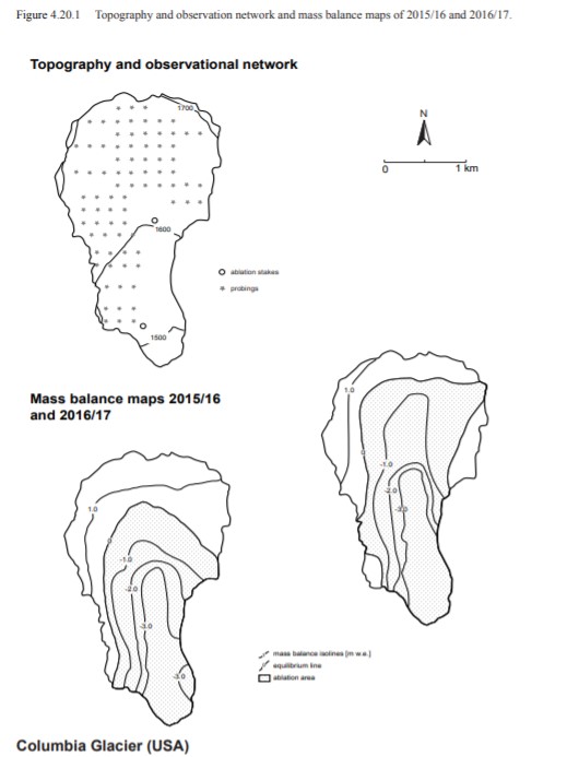
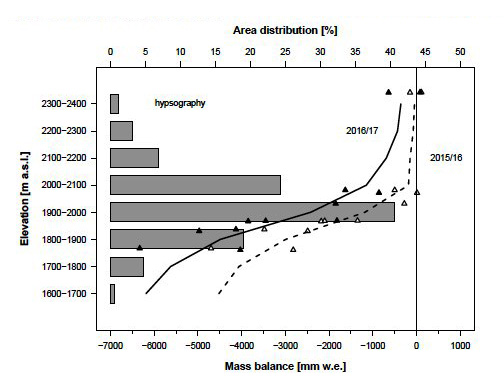
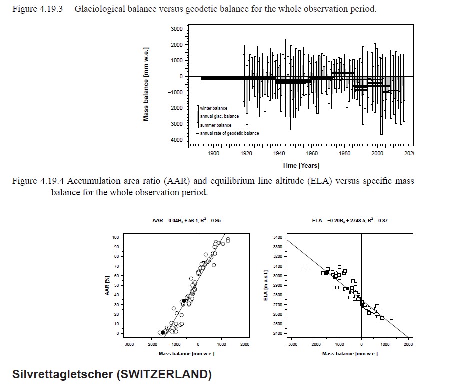
Detailed information is reported for 20 glaciers distributed around the globe that includes annual mass balance maps as illustrated from Columbia Glacier. The relationship between elevatation and annual balance is the balance gradient seen below for Mocho Glacier, Chile. This glacier is in the lake district of Chile at 39.90° S and 72.00° W and did not have significant accumulation in 2016 or 2017.  The  AAR-annual balance relationship and the ELA-annual balance relationship and annual balance record are reported, as exemplied by Silvretta Glacier, Switzerland, where negative balances occurred in 2016 and 2017.

The result of the rising snowline is mass losses, which drives glacier retreat. This also leads to decreased average albedo and surface lowering, which in turn cause pronounced positive feedbacks for radiative and sensible heat fluxes. This rapid decline in mountain glaciers chronicled by WGMS is expected to accelerate.  Huss et al (2017) describe a cascade of effects that are occuring, impacting ecosytems, communites and our economy.

Annual mass balance maps and measurement network on Columbia Glacier.

Annual balance gradient for Mocho Glacier, Chile.

Annual balance record and annual balance relationship to both AAR and ELA on Silvertta Glacier.

Glacier Crevasses As A learning Tool

Guest Post by Clara Deck

Instagram: @scienceisntsoscary


Crevasses on mountain glaciers are large cracks in the ice which often propagate from the surface downward. The initial break will happen when stress exceeds the inherent ice material strength. This article will focus on surface crevasses, though this basic physical understanding also applies to basal crevasses or large-scale rifts in ice sheet and shelf settings.


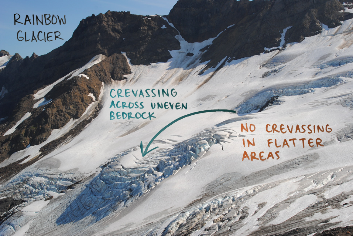
In mountain glacier systems, crevassing is likely to occur as ice flows over bedrock “steps.” Imagine you are baking a pie, and it is time to mold your pie crust to the pan. You must be very careful when bending the dough around the pie pan, because it may crack if you fold it too much or too suddenly.
Glaciers are the same way, and so another driver for crevasse formation is ice flow speed up in these areas. Other factors that could be at play are roughness of the underlying bed or drag along valley walls. The above photo of Rainbow Glacier shows a complex surface of crevassed and smooth areas, which hints to a similarly complex underlying bed.

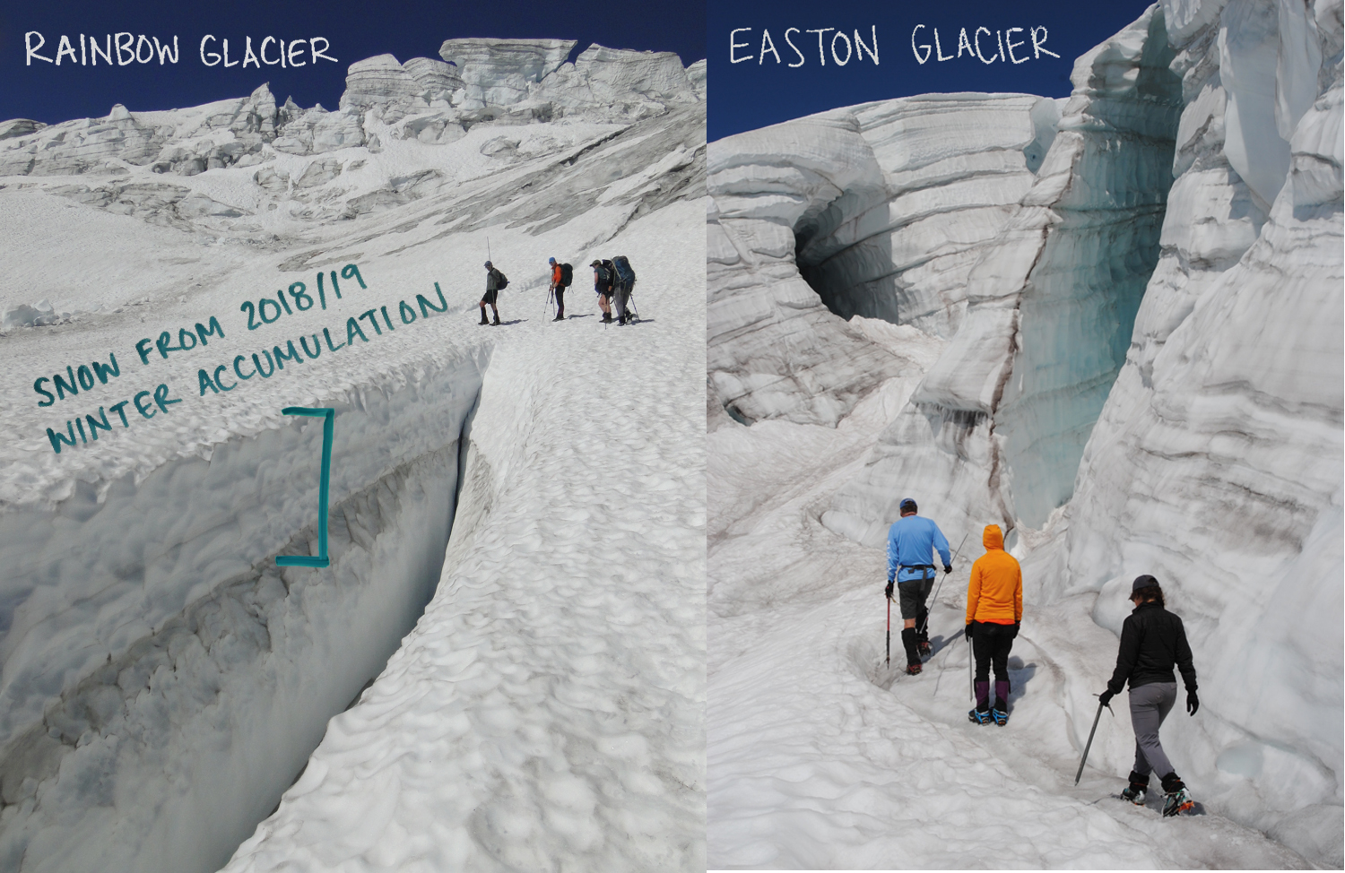
During the 2019 field season of the North Cascades Glacier Climate Project, we measured these crevasses in a few different ways. Seven field seasons ago, Jill Pelto began collecting data on crevasse depth. She uses a cam line, which is essentially a weighted tape measure, to determine total crevasse depth on each glacier. This photo shows Jill measuring a crevasse on Easton Glacier. She tries to analyze crevasses in similar regions of the glaciers from year to year to achieve a cohesive dataset which could be useful on a long-time scale. This data has the potential to shed light on important glacial changes and how they may relate to regional warming or shifts in precipitation patterns in the North Cascades. The data could also illuminate differences in the behavior of each individual glacier. Overall the number of crevasses has declined, in 2019 average depth on Easton Glacier was 10-15 m.

Another technique we used in the field is crevasse stratigraphy. Upon looking inside open vertically-walled crevasses in the accumulation zone, there are clear layers exposed on the crevasse walls. The layers are the remaining snow from each accumulation season, with the most recent winter’s snow on top. Using a rope marked at each decimeter, we work together to measure the depth of each exposed snow layer. These measurements give a pinpointed measurement of mass balance, and thus glacial health, throughout the past couple of years.

In some open crevasse features, you can see that many more years of stratigraphy are preserved, like in this photo on Easton Glacier. Each visible layer is from a year during which the amount of snowfall exceeded the summer melt, and there is no remaining evidence from years with higher melt than snow accumulation.

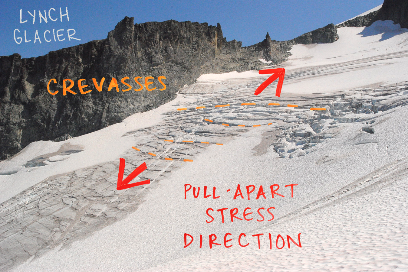
Other information we can gather from crevasses is related to the internal stresses in the ice. Crevasses are opened by pull-apart forces which act perpendicular to the trend of the crevasse.

If you are able to relate the crevasse orientations to the stress within the glacier, it is useful in evaluating the dominant stresses and how they change throughout the glacier spatially. Identifying the locations of crevasse groupings is also a valuable observation, as it reveals the areas with high stress, and may give clues as to where bedrock steps exist below the glacier.

Crevasses are often perceived as scary and have a negative connotation, and while they are hazardous to glacial travelers (always be VERY careful and have the correct gear when navigating crevasses), they are actually a sign of glacial productivity. A healthy glacier’s crevasses are frequent and deep, because thick, flowing ice generates high stress conditions.

The North Cascades Glacier Climate Project has observed glacial thinning due to lower rates of snowfall paired with more intense summer melt seasons over the past 36 years. This has led to a reduction in the number of crevasses in many areas. During summer 2019, the glaciers we visited in the North Cascades will lose up to 2 meters of snow from their surfaces to melting. It is likely that as this pattern continues, there will be even less surface crevassing on the glaciers.

Varied Snowcover Extent Diagnostic of Glacier NP Glacier Climate Response

Snowcover extent in Landsat images from August, 1998 and 2018. S=Sperry, H=Harrison, J=Jackson, B=Blackfoot and P=Pumpelly

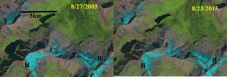
Five of the eight largest glaciers in Glacier National Park are clustered in a small area: Jackson Glacier, Sperry Glacier, Pumpelly Glacier, Harrison Glacier, and Blackfoot Glacier. The USGS in Glacier National Park has over the last 15 years maintained an extensive glacier monitoring program led by Dan Fagre.  This program has led to consistent mass balance observations on Sperry Glacier, and repeat mapping of the 37 named glaciers, 25 of which still qualify as glaciers.  The repeat mapping indicates the area lost from 1966 to 2015, (USGS, 2017).  There is considerable variation between glaciers , some have lost more than 80% of their area and others having lost less than 20% during this 50 year period. Snowcover extent in late summer is a good indicator of glacier mass balance, which controls changes in glacier volume/glacier area.  Glaciers that lack a persistent accumulation zone cannot survive current conditions (Pelto, 2010).  Observations of the snowcover extent in years of limited snowpack illustrate which glaciers do have a persistent snowcover and can survive vs those that cannot (Pelto, 2011). Here we examine Landsat imagery from mid to late August in 1998, 2005, 2015 and 2018, all years of extensive mass loss to identify the difference in snowcover extent, which will drive mass balance loss and subsequent retreat. These images are not at the minimum snowcover extent, which usually occurs n September. For a glacier to be in equilibrium it needs more than 50% of its area to be snowcovered at the end of the melt season.

In 1998 glacier mass balance losses were significant in the region, in mid-August the accumulation area (snowcovered area) on Harrison Glacier exceeded 80%, Blackfoot Glacier was ~60 % snowcovered,  Jackson Glacier ~50% snowcovered and Sperry Glacier ~30% snowcovered.  In 2005 another year of minimum mass balance in the region in late August, Harrison Glacier had ~80% snowcover, Blackfoot Glacier~60% snowcover, Jackson Glacier ~40% snowcover and Sperry Glacier ~20% snowcover. In 2015 glacier volume losses in the region were again large, with Sperry Glacier having a loss of -1.22 m. The retained area of accumulation on Harrison Glacier in mid-August of 2015 was ~60%, on Blackfoot Glacier 50%, on Jackson Glacier 30-40% and on Sperry Glacier less than 20%. In mid-August of 2018 snowcover extent was greater than 75% on Blackfoot, Harrison and Jackson Glacier, while Sperry Glacier had ~40%.

The USGS identified the area of Blackfoot Glacier in 2015 as 1.5 km2, a reduction of 18% from 1966-2015 and 8% from 1998-2015 (USGS, 2017).  Harrison Glacier had an area of 1.7 km2, losing 17% of its area from 1966-2015, and 10% from 1998-2015. Jackson Glacier had an area of 0.8 km2, losing 40% of its area from 1966-2015, and 6% from 1998-2015.  Sperry Glacier had an area of 0.8 km2 in 2015 having lost 40% of its area from 1966-2015, and 16%  from 1998-2015. The persistent pattern of limited snowcover extent on Sperry Glacier indicates why the percentage of area loss has been greater than on the other glaciers. The lack of significant retained snowcover indicates Sperry Glacier cannot survive current climate.  The retention of significant snowcover on Blackfoot and Harrison Glacier even in low snowpack years indicate these glaciers, unlike most in the National Park, can survive the current climate. The Jackson Glacier is in between these two scenarios.

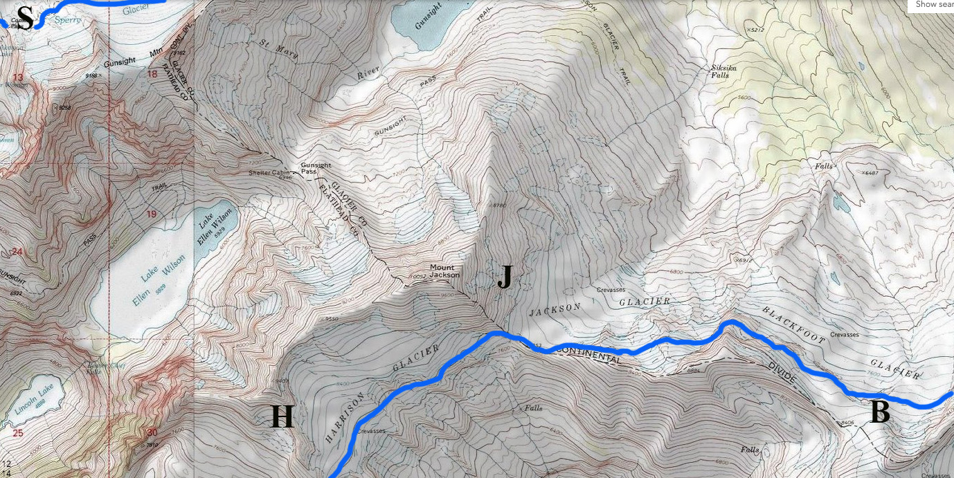
Jackson is the lowest elevation glacier and Harrison is the highest.  Blackfoot, Jackson and Sperry are all north facing. Pumpelly which faces south has lost the least area of the five glaciers from 1998-2015. This underscores the utility of Landsat imagery in assessing glacier mass balance response. Three of the glaciers that retain significant snowcover indicates these glaciers are not as vulnerable to warming and will continue to persist until 2050 at least.

USGS Data on glacier area.

Observation Year LIA 1966 1998 2005 2015
Jackson 3.1 1.3 0.8 0.8 0.8
Harrison 3.5 2.1 1.8 1.7 1.7
Blackfoot 5.0 1.8 1.6 1.6 1.5
Sperry 3.8 1.3 1.0 0.9 0.8

Snow cover extent in Landsat images from August, 2005 and 2015. S=Sperry, H=Harrison, J=Jackson, B=Blackfoot and P=Pumpelly

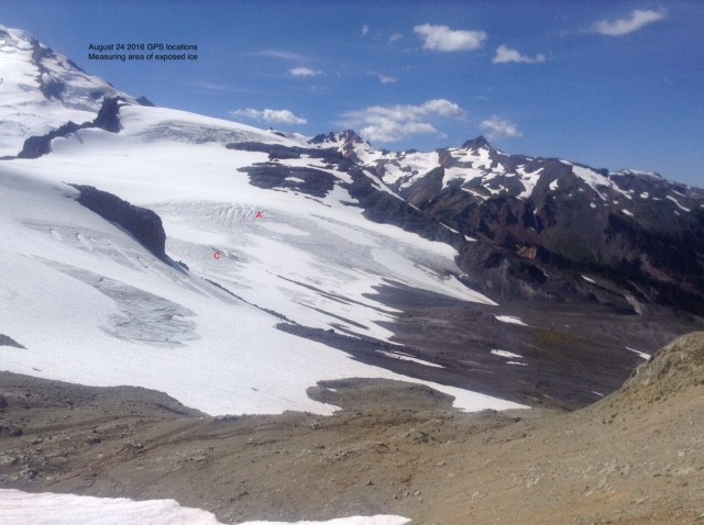
Sholes Glacier August, 24 2016 with the snowcover extent vs the exposed glacier ice.

USGS Topo Map of the area with the blue line indicating the 8000 foot contour.

Drogpa Nagtsang Glacier, China Mass Balance Loss, Separation, Slow Down

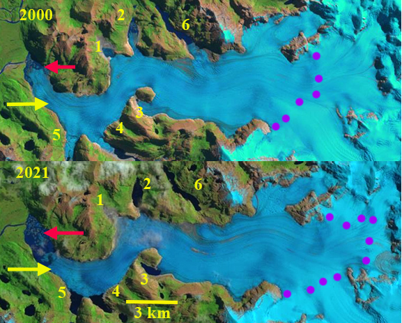
Drogpa Nagtsang Glacier change in Landsat image from 1989 and 2018.  Yellow arrow indicates 2018 terminus location, red arrow 1989 terminus location, red dot the lowest elevation of clean glacier ice. Points A-E are the same locations for comparison.

Drogpa Nagtsang Glacier, China is a glacier that is 30 km west of Mount Everest that terminates in an expanding proglacial lake. The glacier begins on the Nepal border at 6400 m, and its meltwater enters the Tamakoshi River. The Upper Tamakoshi Hydropower project is a 456 MW peaking run of river  is a hydropower project on the Tamakoshi that is to be finished in 2019.  King et al (2017) observed the mass balance of 32 glaciers in the Mount Everest area including Drogpa Nagtsang and found a mean mass balance of all glaciers was −0.52 m water equivalent/year, increasing to -0.7 m/year for lake terminating glaciers. Dehecq et al (2018) in an exceptional paper examined velocity changes across High Mountain Asia from the 2000-2017 period identifying a widespread slow down in the region.  The key take away is the same we see for alpine glaciers around the globe, warming temperatures lead to mass balance losses, which leads to velocity slow down, Mass balance is the key driver in glacier response, a sustained negative mass balance leads to thinning, which leads to a glacier velocity declines whether the glacier is in the Himalaya, Alps or Andes. This study simply could not have been completed without the availability and affordability of Landsat imagery.  Here we look at one example in the region that highlights the important findings.

In 1989 Drogpa Nagtsang Glacier had a substantial number of coalescing supraglacial ponds on its relatively flat stagnant debris covered terminus.  At Point A the former tributary is are no longer contributing to the main glacier, while at B, C, D and E there is a still a contribution.  The snowline in 1989 is at ~5450 m.  The clean glacier ice extends almost to the tributary glacier at Point B at 5200 m, red dot. In 1992 the supraglacial ponds have further expanded, but a true proglacial lake has not formed. The snowline is at~5500 m. Quincey et al (2009) observed flow of less than 10 m/a in lower 5 km of glacier in 1996 and peaking at 20-30 m/a 8 km from terminus. By 2015 a 2.7 km long lake has developed.  The clean glacier ice now extends just past Point E at 5350 m.  The snowline is at 5600 m. The tributaries at Point B, C and E no longer reach the main glacier.  At Point D the medial moraines indicate that flow from this tributary has been reduced and now is a smaller contributor to the valley tongue. In 2018 the clean glacier ice extends to just 5400 m.  The lake has expanded to a length of 2.9 km indicating a retreat of the same distance from 1989-2018.  The snowline is exceptionally high at 5700 m. The former tributaries at B, C and E have also markedly retreated away from the main glacier. Only the tributary at Point D is still contributing to the main glacier. The high snowline observed in recent years are an indication that mass balance losses are even larger in this region, which causes further thinning, reduction in velocity, retreat and expansion of debris cover.  King et al (2018) observed the thinning and velocity profile on Drogpa Nagtsang and noted the velocity decreased over time and was stagnant in the debris covered zone, thinning occurred along the entire profile, which began close to the ELA. The stagnant nature of the terminus tongue is evident in the Digital Globe image below from 2017.  The red arrows show a deeply incised supraglacial stream that is over 2 km long, that would only develop on stagnant ice.  This process has played out on other nearby glaciers such as Yanong Glacier  and Lumding Glacier.  The high snowlines have also been observed at the nearby Nup La on Ngozumpa Glacier in recent years and on many glaciers in the Mount Everest region in recent winters such as in 2018.  This indicates continuing mass losses through a greater period of the year.

Drogpa Nagtsang Glacier change in Landsat image from 1992 and 2015.  Yellow arrow indicates 2018 terminus location, red arrow 1989 terminus location, red dot the lowest elevation of clean glacier ice. Points A-E are the same locations for comparison.

Digital Globe image with yellow dots indicating terminus, red arrows a supraglacial stream, blue arrows ice flow direction.  B is the same tributary has noted in the Landsat images above.

35th Annual Field Observations of North Cascade Glaciers

The 2018 field season observations, conditions and summary. Field team Mariama Dryak, Erin McConnell, Jill Pelto and Mauri Pelto.

For the 35th consecutive year I headed to the North Cascade Range, Washington to monitor the response of glaciers to climate change.  Two of the glaciers the North Cascade Glacier Climate Project (NCGCP) monitors are now part of the 42 glaciers comprising the World Glacier Monitoring Service  (WGMS) reference glacier network, where annual mass balance has been assessed for more than 30 years consecutively.

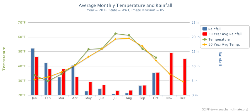
The 2018 winter season featured relatively normal snowpack despite a winter of wide temperature fluctuations, February freezing levels 400 m below the mean and December 500 m above the mean. Summer melt conditions featured temperatures 1.1 C above the 1984-2017 mean. The summer melt season through August was warm and exceptionally dry, which has also helped foster forest fires. The melt rate during the August field season was 35% above normal.

Washington Climate Division Five, western North Cascades

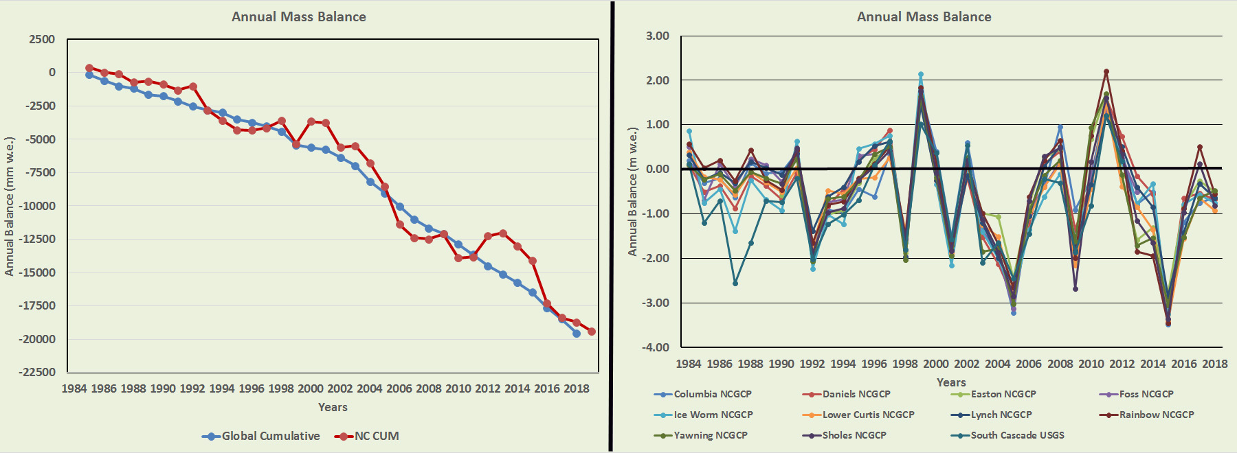
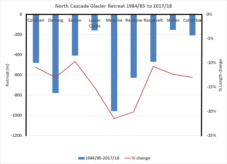
We assessed the mass balance of eight glaciers.  All eight will have significant negative mass balances in 2018, between -0.5 m and -1.0 m.  Retreat was measured on seven of the glaciers where the terminus was exposed, all had retreated since 2017 with the retreat ranging from 7-21 m. This continues the pattern of significant retreat each year that began in 2014. The overall length loss as a percentage of total length falls into a relatively narrow range of 10-22%.  The mass balance losses has also led to additional rock outcrops emerging in what had been the elevation of the accumulation zone.  We continued to measure runoff below Sholes Glacier and to assess crevasse depth.  The average crevasse depth in 2018 was 10 m, with the deepest at 16 m on Lower Curtis Glacier.

Annual  mass balance of North Cascade glaciers 1984-2018 (right).  Cumulative glacier mass balance from NCGCP compared to WGMS global cumulative mass balance.  Below is the retreat of selected North Cascade glaciers during the last 35 years, in meters and as a percentage of the total length.  Locations for all but Columbia Glacier are in image below. 

Mount Baker and Mount Shuskan glaciers identified in a Landsat image from 8-9-2018. Blue indicates mass balance and terminus change are observed.  Orange indicates only terminus change is observed. C=Coleman, D=Deming, E=Easton, LC=Lower Curtis, M=Mazama, N=Nooksack, P=Price, R=Rainbow, Rv=Roosevelt, SH=Sholes. 

Major Late July Meltdown on Lowell Glacier, Yukon

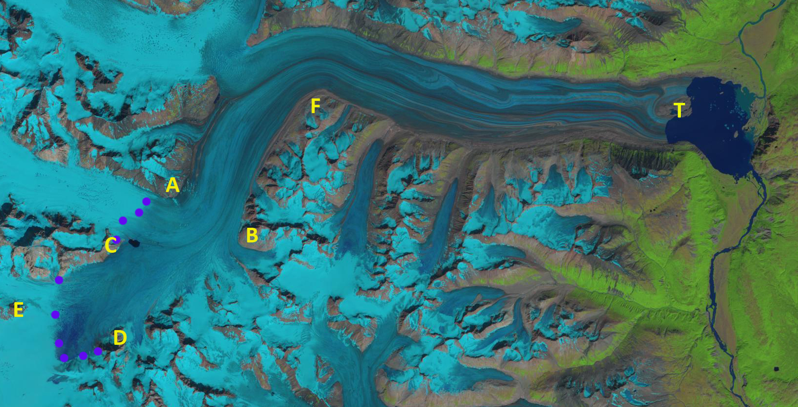
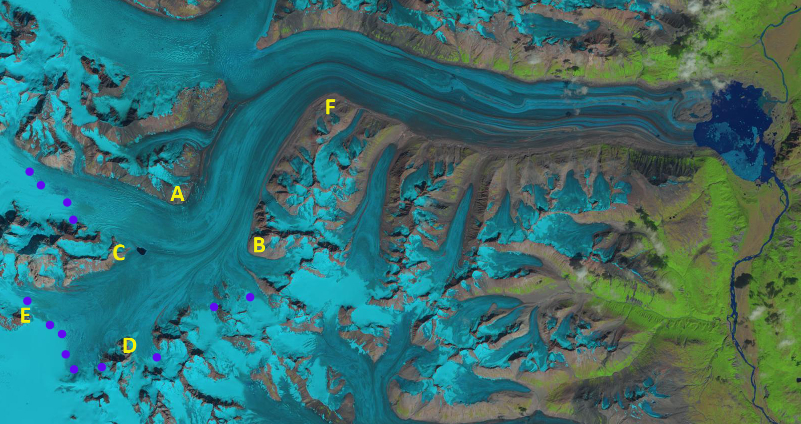
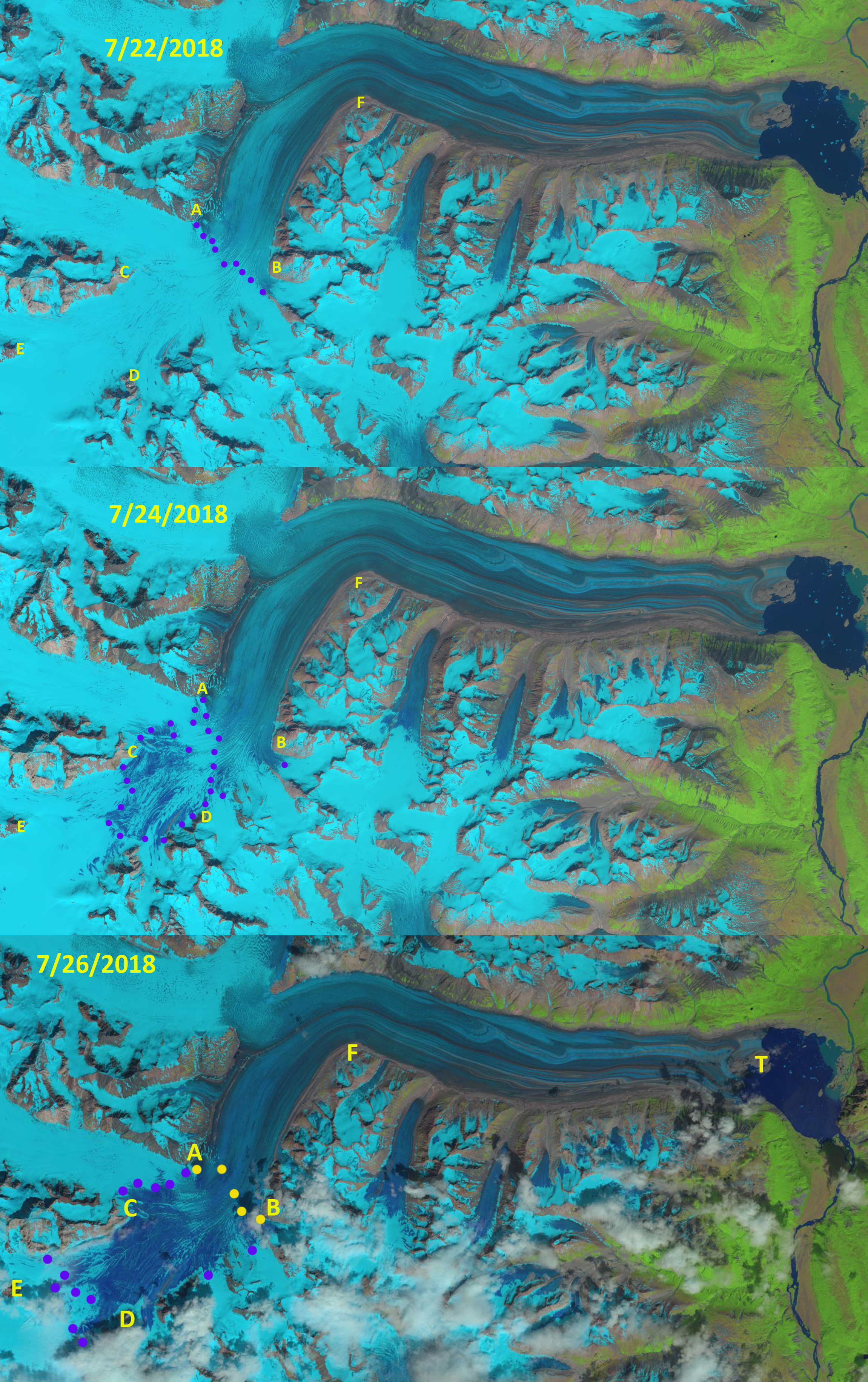
Lowell Glacier in Landsat images from 7/4, 7/26 and 8/11 with Sentinel images from 7/22 .  The snowline is shown with purple dots. Point A-F are fixed reference locations.  The snowline migrated upglacier 20 km and 300 m in elevation.  A significant snow swamp is between the yellow and purple dots on 7/26, that was not present on 7/22. 

The Lowell Glacier drains east from the St.Elias Range on the Yukon-Alaska border.  A sequence of images from July 4-Aug. 11 indicate the rapid snowline rise, with a particularly rapid transition from July 22-July 26.  During this period weather records from Haines Junction, Yukon indicate daily high temperatures of:  7/22=29.5 C, 7/23= 28.1, 7/24=26.8, 7/25=25.5, 7/26=25.1. This equates to project freezing levels above 4200 m each day.

(NASA Post follow up to this research)

On July 4th the transient snowline on Lowell Glacier was near Point F at 1240 m.  By July 22 the transient snowline had moved 9 km upglacier to 1400 m between Point A and B. Just two days later the region from 1400-1560 m an area of 40+square kilometers was under rapid transition with the snowline rising and an area of slush developing, saturated snowpack, really a “snow swamp”.  By July 26th the slush line was at 1520 to 1560 m, with the slush indicated by a royal blue color distinguishing it from the graying blue bare ice or old firn, and the white blue snow from the previous winter than was not fully saturated with water.  It is unusual to develop such a large “snow swamp” so quickly, this was accomplished by the rapid ablation due to the high temperatures. By Aug. 11th the transient snowline had shifted above this slush zone, with all of the saturated snow having ablated away, to Point E at 1560-1600 m.  The snowline in late summer of 2010, 2015 and 2017 also reached near Point E at an elevation of 1520-1600 m.  In 2015 and 2017 a supraglacial lake developed just east of Point C.  Another good example of a large snow swamp is in Svalbard on Hinlopenbreen. Taku Glacier, AK had the highest snowline in over 70 years of observation in 2018.

If a good image is acquired in September I will add to this post.  The consistently high late summer snowline, above 1500 m cannot sustain the Lowell Glacier, which will drive further retreat.  The retreat of this glacier be both enhanced and mitigated by surges, during the surge cylcle.  The glacier has surged five times since 1948 (Bevington and Copland, 2014).  The surge cycle has been getting shorter and will not offset the overall mass loss that will drive retreat, just as has occurred on Svalbard glaciers.

Sentinel from 7/22, 7/24 and Landsat from 7/26 indicating the change in snowline and snow swamp development, purple dots.  T indicates terminus of glacier.

Landsat image from 8/8/2017 indicating snowline near Point D and E at m on Lowell Glacier.

Landsat image from 8/3/2015 indicating snowline near Point D and E at m on Lowell Glacier.

Landsat image from 9/14/2010 indicating snowline near Point D and E at m on Lowell Glacier.


Alpine Glacier-BAMS State of the Climate 2017

Global alpine glacier annual mass balance record of reference glaciers submitted to the World Glacier Monitoring Service, with 2017 continuing the trend of significant negative mass balance. 

The Bulletin of the American Meteorological Society: State of the Climate 2017 has been published.  Since 2008 I have written the chapter on alpine glaciers.

The World Glacier Monitoring Service (WGMS)record of mass balance and terminus behavior (WGMS 2017) provides a global index for alpine glacier behavior. Glacier mass balance is the difference between accumulation and ablation, reported here in mm of water equivalence. Mean annual glacier mass balance in 2016 was −847 mm for the 37 long-term reference glaciers and −761 mm for all 140 monitored glaciers. Of the reporting reference glaciers, only one had a positive mass balance. Preliminary data reported to the WGMS in 2017 from Austria, Canada, China, France, Italy, Kazakhstan, Norway, Russia, Switzerland, and United States indicate that 2017 will be the 38th consecutive year of negative annual balances with a mean loss of −1036 mm for 29 reporting reference glaciers, with three glacier reporting a positive mass balance (http://wgms.ch/latest-glacier-mass-balance-data/).

The ongoing global glacier retreat is currently affecting human society by raising sea levels, changing seasonal stream runoff, and increasing geohazards (Huss et al. 2017a). Huss and Hock (2018) indicate that approximately half of 56 glaciated watersheds globally have already passed peak glacier runoff. Rounce et al. (2017) identify the widespread expansion of glacier lakes due to retreat in Nepal from 2000 to 2015, which pose a glacier lake outburst flood hazard. Glacier retreat is a reflection of strongly negative mass balances over the last 30 years (Zemp et al. 2015). Marzeion et al. (2014) indicate that most of the recent mass loss, 1991–2010, is due to anthropogenic forcing.

The cumulative mass balance loss from 1980–2016 is −19.9 m, the equivalent of cutting a 22-m thick slice off the top of the average glacier .  The trend is remarkably consistent from region to region (WGMS 2017). WGMS mass balance based on 41 reference glaciers with a minimum of 30 years of record is not appreciably different from that of all glaciers at −19.1 m. The decadal mean annual mass balance was −228 mm in the 1980s, −443 mm in the 1990s, −676 mm for 2000s, and –896 mm for 2010–17 (WGMS 2017). The declining mass balance trend during a period of retreat indicates alpine glaciers are not approaching equilibrium and retreat will continue to be the dominant terminus response.

Exceptional glacier melt was noted across the European Alps, leading to high snowlines and contributing to large negative mass balance of glaciers on this continent (Swiss Academy of Sciences 2017). In the European Alps, annual mass balance has been reported for nine reference glaciers from Austria, France, Italy, and Switzerland. All had negative annual balances: exceeding −1000 m with a mean of −1664 mm. This continues the pattern of substantial negative balances in the Alps that continue to lead to terminus retreat. In 2016, in Switzerland 94 glaciers were observed: 82 retreated, 7 were stable, and 5 advanced (Huss et al. 2017b). In 2016, Austria observed 90 glaciers: 87 retreated, 2 were stable, and 1 advanced; the average retreat rate was 14 m (Fischer 2017).

In Norway and Svalbard, terminus fluctuation data from 36 glaciers with ongoing assessment, indicates that in 2016 32 retreated, 3 advanced, and 1 was stable. The average terminus change was −12.5 m (Kjøllmoen, 2017). Mass balance surveys with completed results are available for nine glaciers; seven of the nine had negative mass balances with an average loss of −80 mm w.e.

In western North America data have been submitted from eight reference glaciers in Alaska and Washington in the United States, and British Columbia in Canada. Seven of the eight glaciers reported negative mass balances with a mean loss of −1020 mm. Winter and spring 2017 had above-average snowfall, while ablation conditions were above average. In Alaska mass losses from 2002 to 2014 have been −52 ± 4 gigatons yr−1, as large as any alpine region in the world (Wahr et al. 2016).

In the high mountains of central Asia four glaciers reported data from China, Kazakhstan, and Nepal. All four were negative, with a mean of −674 mm. This is a continuation of regional mass losses, such as reported by King et al. (2017) who found for 2000–15 the mean annual mass balance of 32 glaciers in the Mount Everest region was −520 ± 220mm.


Landsat image from 8/19/2017 illustrating the snowline on Mont Blanc glaciers with one month left in the melt season (M=Mer de Glace, A=Argentière, S=Saleina, L=Le Tour, T=Trient)


How Unusual Was 2015 in the 1984–2015 Period of the North Cascade Glacier Annual Mass Balance?

Sholes Glacier during the first week of August 2015 versus and average year such as in 2017.  Note stream gage and weather station at this site. The greater extent of bare ice enhances ablation as for a given temperature there is a higher ablation rate for ice then snow. Columbia Glacier a WGMS reference glacier viewed from above the glacier at Monte Cristo Pass at the start of August in 2015 and 2016.  Note the lack of retained snow in 2015 and the multiple firn layers exposed. 

This post is a shortened version of the publication out this week in Water.

In 1983, the North Cascade Glacier Climate Project (NCGCP) began the annual monitoring of the mass balance on 10 glaciers throughout the Washington mountain range, in order to identify their response to climate change. Annual mass balance (Ba) measurements have continued on seven original glaciers, with an additional two glaciers being added in 1990. The measurements were discontinued on two glaciers that  disappeared and one was that separated into several sections. This comparatively long record from nine glaciers in one region, using the same methods, offers some useful comparative data in order to place the impact of the regional climate warmth of 2015 in perspective.  This led to the most negative annual balance of the last 26 years on every glacier.

2015 Climate

The 2015 winter accumulation season featured 51% of the mean (1984–2014) winter snow accumulation at six long-term USDA SNOTEL stations in the North Cascades, namely, Fish Creek, Lyman Lake, Park Creek, Rainy Pass, Stevens Pass, and Stampede Pass. This was exceptional as it was the second lowest out of the 32 years of the mass balance observation series. The winter season was exceptional for warmth, being the warmest winter season on record in the state of Washington. The freezing level in 2015 averaged 1645 m in the Mount Baker region from November–March, compared with an average of 1077 m (John Abatzoglou, Freezing Level Tracker). The previous record for the mean November–March freezing level, since the record began in 1948, was 1500 m.

Freezing Level November-March on Mount Baker, WA from Freezing Level Tracker 1948-2017.

In 2015, the mean May–September temperature at Diablo Dam was 2.2 °C warmer than the long term mean, and it was the second warmest to 1958 in the 1950–2015 record. For June–September, the mean temperature was 2.0 °C warmer than the long term mean, and was also second to 1958 as the warmest. The combination of the warmest melt season in over 50 years and the second lowest accumulation season snowpack in the last 30 years was a good indication that the glacier mass balance would be quite negative.
In 2015, the sea surface temperature waters that had developed in the winter of 2013/14, persisted off the coast of the Pacific Northwest, with anomalies generally exceeding 2 °C (Di Lorenzo and Mantua, 2016)

Glacier Mass Balance 2015

The mean annual balance of the NCGCP glaciers is reported to the World Glacier Monitoring Service (WGMS), with two glaciers, Columbia and Rainbow Glacier, being reference glaciers.  The mean Ba of the NCGCP glaciers from 1984 to 2015, was −0.54 m w.e.a−1 (water equivalent per year), ranging from −0.44 to −0.67 m w.e.a−1 for individual glaciers. In 2015, the mean Ba of nine North Cascade glaciers was −3.10 m w.e., the most negative result in the 32-year record. The correlation coefficient of Ba was above 0.80 between all North Cascade glaciers, indicating that the response was regional and not controlled by local factors. In 2015, out of the nine glaciers where the Ba was examined, the AAR was 0.00 on seven of the glaciers, 0.05 on the Rainbow Glacier, and 0.26 on the Easton Glacier. For each glacier, the 2015 Ba was the most negative of any year in their entire record. The South Cascade Glacier had a negative mass balance of −2.72 m w.e. in 2015, which was the most negative Ba reported since the suite of continuous mass balance measurements began in 1959 [USGS, 2017].  The probability of achieving the observed 2015 Ba of −3.10 is 0.34%.

 
Annual mass balance of North Cascade glaciers, note the similar annual response indicating regional climate conditions are the overriding driver of mass balance. 

On June 15, when the automatic weather station and discharge station were installed adjacent to the Sholes Glacier, the snowpack was similar to a typical early August snow cover. On the Sholes Glacier, the AAR fell from 0.55 on 9 July to 0.00 on 9 September. This was the first year since the monitoring had begun in 1984 that the mean AAR in early August was below 0.25. The result was an exposure of the older firn layers and a general decrease in albedo. In early August, the AAR was below 0.1 for all of the glaciers, except for the Easton Glacier. On the Columbia Glacier, the AAR on August 1 was the lowest observed yet at 0.12, with six weeks remaining in the melt season. The early exposure of glacier ice was important as the melt rate was faster, as was indicated by the greater melt factor.  The North Cascade mass balance cumulatively over the last 30 years matches closely the global mean mass balance loss.

Map of North Cascade glaciers observed in this study. 

Comparison of North Cascade cumulative and Global cumulative glacier mass balance


Lower Curtis Glacier Annual Terminus Response to Climate Change

Side view of Lower Curtis Glacier in 2013, 2015 and 2017, illustrating the reduced slope and height of glacier front in just four years.

Terminus observations have been reported to the WGMS from 2500 glaciers with 46,500 specific observations since the late 19th century, which you can explore with the glacier viewer application. Here we examine what it looks like to report from a glacier each year.  I have visited this glacier 34 consecutive years, each time camping in a tent near the glacier, a fun spot indeed when the weather cooperates. The Lower Curtis Glacier is an avalanche fed cirque glacier on Mount Shuksan in the North Cascades of Washington. It is a south facing and low elevation glacier for the range. This is an unusual combination that is supported by the heavy accumulation via avalanching from the upper slopes of Mount Shuksan. The glacier displays a magnificent set of annual layers in its terminus tongue. The terminus tongue is a spectacular wall of seracs that quickly rises 55 m above the bedrock. There are typically 50 layers visible indicating that this most of the ice in the glacier is 50 years of less in age.

Lower Curtis Glacier Front in 2007 and 2017 taken from same location.  Both retreat and thinning of the front in the decade is evident. 

From 1908 to 1950 the glacier retreated from the valley bottom into the cirque. The glacier advanced from 1950-1985 down slope and has retreated since.  Each year we survey the terminus location, measure the mass balance and survey the glacier surface elevation on a cross profile. Here we report on the annual terminus survey from 2007-2017.  The frontal change reported to the World Glacier Monitoring Service has been 2007=-13 m, 2008=-17 m, 2009=-20 m, 2010=-7 m, 2011=-5 m, 2012=-6 m, 2013=-5 m, 2014=-12 m, 2015=16 m, 2016=-16 m and 2017=12 m. This is a total of 129 m of retreat in 11 years, nearly 12 m per year. A longitudinal profile up the middle of the glacier indicates that it thinned 30 meters from 1908-1984 and 22 m from 1985-2016. Because of its heavy accumulation via avalanching the glacier moves rapidly and is quite crevassed at the terminus with large high seracs at the glacier front. In 2007 the height of the terminus seracs was 45 m, by 2014 the seracs were 37 m high and in 2017 had shrunk to 26 m high and not as steep.  The imposing tongue has certainly diminished. The glacier retreat fits the pattern in the region, with all Mount Baker a glaciers retreating (Pelto, 2015).

From a Glaciologists Perspective AGU Day 3

Snapshot of day 3  of Glaciology poster presentations at AGU.  The amount of glaciology research is impressive, there is much we do not know.  We can no longer say that we know very little about any aspect or region.  Before saying that explore the vast literature that is now available.

Jeff La Freniere at Gustavus Adolphus College used several new technologies,  aerial and terrestrial LIDAR and structure-from-motion photogrammetry from drones make mass balance measurements using geodetic approaches increasingly feasible in remote mountain locations like Volcán Chimborazo, Ecuador. The result combined with a unique, 5-meter resolution digital elevation model derived from 1997 aerial imagery, reveal the magnitude and spatial patterns of mass balance behavior over the past two decades. Above are the results they found more specifically that on the Hans Meyer Glacier terminus, the mean surface elevation change since 1997 has been nearly 3 m yr-1, while on the lower-elevation Reschreiter Glacier the mean elevation change has been approximately 1 m yr-1 .

Aurora Roth, University of Alaska Fairbanks  developed and applied a linear theory of orographic precipitation model to downscale precipitation to the Juneau Icefield region over the period 1979-2013. This LT model is a unique parameterization that requires knowing the snow fall speed and rain fall speed as tuning parameters to calculate cloud time delay. The downscaled precipitation pattern produced by the LT model captures the orographic precipitation pattern absent from the coarse resolution WRF and ERA-Interim precipitation fields. Key glaciological observations were used to calibrate the LT model. The results of the reference run showed reasonable agreement with the available glaciological measurements, which is what glacier mass balance observations have shown. The precipitation pattern produced was consistent regardless of horizontal resolution, and climate input data, but the precipitation amount varied strongly with these factors.  The import is to help model mass loss from glaciers in Southeast Alaska which will alter downstream ecological systems as runoff patterns change. 

Joanna Young, University of Alaska Fairbanks  focuses on partitioning GRACE glacier mass changes from terrestrial water storage changes both seasonally and in long-term trends using the Juneau Icefield, which has long term glacier mass balance data, as a case study for . They leverage the modeling tool SnowModel to generate a time series of mass changes using assimilated field observations and airborne laser altimetry, and  compare to GRACE solution from the NASA Goddard Space Flight Center Geodesy Laboratory .  This is one of the first to analyze GRACE at the sub-mountain range scale, and to examine terrestrial water storage trends at a smaller scale than the full Gulf of Alaska. The figure above looks at subannual and long-term changes of the Juneau Icefield from 2003 to present.

Emilio Ian Mateo, University of Denver  Looked at rock glaciers in the San Juan Mountains of Colorado examining how slope aspect and rising air temperatures influenced the hydrological processes of streams below rock glaciers. Detailed findings  illustrated above from 2016 and 2017 show that air temperature significantly influenced stream discharge below each rock glacier. Discharge and air temperature patterns indicate an air temperature threshold during late summer when rock glacier melt increased at a greater rate. The results suggest that slope aspect influences stream discharge, but temperature and precipitation are likely the most components of the melt regimes. 

Maxime Litt, Utrecht University installed an eddy-correlation system (Campbell IRGASON) during a period of 15 days over the Lirung glacier in the Langtang Valley in Nepal , during the transition period between the monsoon and the dry season to examine surface energy balance.  Results are also reported from Mera Glacier and Yala Glacier. At Lirung Glacier during the day, moderate winds blow up-valley and the atmospheric surface layer is unstable. Latent (sensible) heat fluxes scale between 50 and 150 (50 and 250) Wm– 2 during the day, thus drying and cooling the debris and significantly impact SEB. At night, weak down-glacier winds are observed and fluxes remain weak. Yala and Mera Glacier are different environments and illustrate the variations in position on SEB.

Katherine Strattman, University of Dayton reported on a study of the  Imja, Lower Barun, and Thulagi Glaciers in the Nepal Himalaya. The retreat of the glaciers has led to proglacial lakes continuing to dramatically increase in area. They used Landsat, ASTER, and Sentinel satellite imagery to study the conditions of these glaciers. They assessed interannual changes in surface ice velocity from the early 1990s to present. They found both long-term and short-term velocity variations.  Satellite imagery indicates the three lakes exhibit three contrasting trends of lake growth: Imja Lake has a strong accelerating growth history since the 1960s, Lower Barun a very slow accelerating growth, and Thulagi a decelerating growth, even as the glaciers of all three lakes have thinned. Above is the velocity of Barun Glacier showing velocity changes and growth of the lake.

Shashank Bhushan, Indian Institute of Technology Dhanbad developed a hazard assessment of  moraine dammed glacial lakes in Sikkim Himalayas. They generated high-resolution DEMs using the open-source NASA Ames Stereo Pipeline (ASP) and other open-source tools to calculate surface velocity and patterns of glacier downwasting over time. Geodetic glacier mass balance was obtained for three periods using high-resolution WorldView/GeoEye stereo DEMs, Cartosat-1 stereo DEMs and SRTM. Initial results revealed a region-wide negative annual mass balance of -0.31± m w.eq. for the 2007-2015 period. 

From a Glaciologists Perspective AGU Day 2

It has been 30 years since my first experience at the AGU, at that time glaciology and the cryosphere played a small role.  Today that is clearly not the case.  Today just a glimpse of a few of the many interesting glaciers studies are provided to again illustrate the vast array and amazing detail of work being conducted.

Samiah Mustafa, Brown University presented research looking at the ability of a melt model to generate accurate discharge at three watersheds in West Greenland; North River (Thule), Watson River (Kangerlussuaq), and Naujat Kuat River (Nuuk). In each watershed they modeled melt at daily, 5, 10 and 20 day time scales.  They found Nuuk and Thule basins did not do well at a daily time scale, but do capture variability over 5-, 10-, and 20-day means (r2 > 0.7). Results at Watson River were in good agreement at each time scale. Model agreement with river flow data  is reduced during periods of peak discharge, particularly for the exceptional melt and discharge events of July 2012 evident in chart above.

Waldemar Walczowski, Institute of Oceanology Polish Academy of Sciences reported on a study combining glacier retreat and examination of water temperatures in the Hornsund fjord (southern Svalbard), collected under the Polish-Norwegian projects GLAERE and AWAKE-2.  The observed direct contact of warm oceanic water with a glacier’s calving face enhances submarine melting, undercutting and glacier calving.  The turbulent plumes of subglacial meltwater were key in heat transfer and influence glacier retreat. 

Martin Wearing from Lamont Doherty examined the development of crevasses in the past as the Ronne Ice Shelf advanced over the Henry Ice Rise.  The ice shelf thickened and advanced coming in contact with the bedrock high and generating crevasses that first formed around 600o years ago.  They discovered the featured in radar profiles of the ice shelf.  The sequence of crevasse development is seen above.

Morgan Whitcomb from University of Michigan used a simple damage evolution law, based on crevasse distributions as a continuum field to yield estimates of ice shelf calving rates when combined with the Community Ice Sheet Model (CISM).  Their basal melt function enhanced crevasse growth near the ice shelf terminus, leading to increased iceberg calving.  The diagram above shows the model predicts broadly correct calving rates for ice tongues ranging in length from 10 km  on Erebus to over 100 km  on Drygalski Glacier.


Ann Hill, Skidmore college working with the Juneau Icefield Research Programs velocity monitoring program reports on a comparison of velocity and surface elevation on Taku Glacier from 1997-2017.  The velocity on the main profile was consistent, as it had been back to 1950.  The surface elevation has experienced thinning after 1997 after a prolonged period of thickening.  Above are three velocity profiles with red and blue arrows from 1997 and 2017 mostly overlaying each other because velocity did not change.  Above are profiles of height changes for various periods.

 Lu An from UCal Irvine used multiple sources to reconstruct bathymetry glacier bed topography near the grounding line of Sermeq Avangnardleq (AVA) and Sermeq Kujatdleq (KUJ) in central West Greenland.  They used high resolution airborne gravity data from AIRGrav and MultiBeam Echo Sounding data collected in the fjord. The seamless topography obtained across the grounding line reveal the presence of a 300-m sill for AVA that has stabilized its terminus.  For KUJ shown above the sill has helped stabilize the glacier though it has still retreated ~1 km and has led to iceberg stranding.