Visualizing Glacier Melt Impacts

On September 4, 2015May 2, 2024 By mspeltoIn glacier climate change, Glacier Observations, glaciers salmon, North Cascade Glaciers1 Comment

Key questions emerge from the summer of 2015 in the Pacific Northwest glacier basins. That can both be visualized and quantified.

With record temperatures and minimum flows in most rivers in the Cascade Range during July and August of 2015, a key question was how much did glaciers contribute in basins that are glaciated? Note the water pouring off the glacier and the lack of snowcover in the first few minutes of the video.

You can examine flow per unit watershed area as a first order observation. In the unglaciated South Fork discharge was 0.5 cfs/square mile, rising to 0.7 cfs/square mile in the lightly glaciated Skykomish River and 4.3 cfs/square mile in the heavily glaciated North Fork Nooksack. For a more direct measure we measured ablation from July 29 to August 17th in the North Fork Nooksack and Skykomish River basin. With the Nooksack Tribe we also measured discharge below glaciers in the North Fork but those recorders are still deployed in the field.

Because the glaciers had mostly ice, not snow at the surface, melting was enhanced. We found in the Skykomish Basin that glacier runoff was 45 CFS versus a mean discharge of 375 CFS , this is 12% of the total flow despite covering only 1.3 % of the basin. In the North Fork Nooksack glacier runoff was 340 CFS versus total flow of 460 CFS, this is 74% of the total flow though only 6.1 % of the basin has glacier cover. In both cases the glaciers contributed a river flow percentage 12 times greater than the percent of basin area they cover. With a substantial loss in glacier area occurring this summer, next year glacier runoff for the given climate conditions will be reduced. Given this higher flow the glacier fed streams offer less stressful conditions this summer to salmon.

How much did glacier runoff water temperature amelioration?

In the South Fork Nooksack without glaciers stream temperature was above 20 C on eight days between Aug.1 and Aug. 20. In the North Fork Nooksack with glacier contribution, the stream temperature peaked at 13-14 C.

With the early loss of snowcover and exposure of the underlying ice, how are glacier ice worms impacted? In the video note ice worms featured in the first minute in a glacier filled crevasse.

These worms live on snow algae primarily, which would seem to be in short supply in a summer with limited snowpack on the glaciers. How well can they survive being on the glacier ice for extended periods? For the 21st year we conducted ice worm population surveys. The numbers were the lowest we have seen at 175-250 ice worms per square meter, but it should be next year when the full impact would be evident.

How much glacier area will be lost? Note the visual of terminus retreat.
The summer is not over, but our observations indicate a 5-7 % volume loss will occur. This should be approximately equaled by area loss. Hopefully good satellite imagery in September will provide a specific answer. The Aug. 17th Landsat image is excellent. Retreat just this summer has been 40 m on Easton Glacier, 32 meters on Columbia Glacier, 25 meters on Sholes Glacier and 30 meters on Lower Curtis Glacier.

Aug. 17 Landsat image. Arrows indicate areas where we observed rapid area loss of glacier ice this summer.

Mount Caubvick Glacier Retreat, Labrador

On September 1, 2015May 2, 2024 By mspeltoIn Canada glacier retreat, climate change glacier retreat, glacier climate change, Glacier Observations

Mount Caubvick is in the Torngat Mountains of Labrador 35 km inland of the Atlantic Ocean and south of Nachvak Fjord. Way et al (2014) identified 105 active glaciers that had flow indicators in these mountains. The mean elevation of these glaciers is quite low at 776 meters above sea level. The radiational shading and higher accumulation from protected cirque locations and proximity to the ocean are key to the low elevations. The elevation of the glaciers around Mount Caubvick is higher. Here we use Landsat images from 1992, 1997 and 2015 to identify response to climate change. The annual layers preserved in the glacier ice are evident in glacier B,C and E.

2013 Google Earth image of Mount Caubvick, Torngat Mountains, Labrador.

In 1992 Glacier A terminates at the red arrow in an expanding lake. Glacier C terminates at the yellow arrow in a just forming glacial lake. Glacier E terminates at the purple arrow in a glacial lake that is similar in length to the glacier. In 2015 each lake has notably expanded. The arrows are in the same locations in the 2015 image. At the red arrow, Glacier A has retreated 200 m, which is 20% of its entire length. Glacier C, yellow arrow has retreated 250 m, 40% of the total glacier length. At the purple arrow, Glacier D has retreated 225 m, which is 35% of its total length. The retreat of Glacier B and E is less clear as the terminus locations are hard to determine in 1992. What is most evident is the reduction in ice area at the higher elevations of the glaciers noted by the green arrows. In 1997 there is little expansion of the three lakes since 1992, indicating most of the retreat has been in the last 18 years. Glacier B provides a good snapshot of annual layers. The black arrow indicates the lack of an accumulation zone, without which a glacier cannot survive (Pelto, 2010). The red arrow indicates a band of annual layers that marks what had been the typical snowline Indeed none of the glaciers in 2015 in either the 2013 Google Earth image or 2015 Landsat have significant retained accumulation, indicating none can survive current climate. Way et al (2014) figure 4 indicates an example of the same snowline setup on a different glacier near Ryans Bay. . it is evident that in the last decade firn and snow are not retained consistently. Sharp et al (2014) indicate in Figure 52 the mass loss of Canadian Arctic glaciers in general, that parallels that of Labrador.

1992-2015 Landsat comparison of Mount Caubvick glaciers

Glacier B with numerous annual layers with the snowline indicates by red arrow and lack of accumulation black arrow.

Glacier C annual layers.

Barskoon Mountain Glacier Widespread Retreat, Tien Shan Range, Kyrgyzstan

On August 26, 2015May 2, 2024 By mspeltoIn climate change glacier retreat, glacier climate change, Glacier Observations

Farinotti et al. (2015) used three approaches to assess glacier change in the Tien Shan from 1961 to 2012. The results converge on an overall loss of glacier area of 19-27%,a spatial extent of 2960 square kilometers of glacier area. They further observe that it is primarily summer melting that has driven the change. Here we examine the change of several glaciers in a small sub-range in the Barskoon Mountain area of Kyrgyzstan using Landsat images from 1990-2013.. The A364 road extends up the Barskoon valley and was part of the silk road. It is now more widely used as the main road to the Kumtor Gold Mine (Colgan, 2015).

Google Earth image of Tien Shan Mountains and glaciers in Kyrgyzstan, study area is Barskoon Mountains.

In 1990 working clockwise from the black arrow, which indicates two glaciers merging and then ending in a proglacial lake. At the green arrow is a third glacier that now terminates short of this developing lake. At the yellow arrow a fourth glacier terminates in a small proglacial lake. At the purple arrow a glacier ends in a valley lacking any lake. At the red arrow the glacier expands into a broad terminus lobe in a valley with two small lakes both north and south of the terminus. By 1997 the lake at the black arrow has extended as the glacier terminating in it has retreated. The glacier at the green arrow terminates further from the lake. At the red arrow the terminus lobe is much thinner. By 2013 the two glaciers that terminated in the lake have now receded from the lake with a total retreat of 400-500 m since 1990. At the green arrow the glacier now terminates 600 m from the lake instead of 300 m in 1990. At the yellow arrow the glacier no longer reaches the lake it had terminated in. At the purple arrow a new 200 m long lake has formed. The most dramatic change is at the red arrow where the terminus tongue is only 30% of the area it was in 1990. All of these are unnamed glaciers, and each like those adjacent without arrows indicating specific changes have been retreating and losing area. The typical length of these glaciers is 2-4 km, and those indicated have lost at least 10% of their length from 1990 to 2013. This is a sustained loss of mass balance, on glacier that do not experience any calving losses. The changes are similar for larger glaciers in the Tien Shan such as Petrov Glacier.

1990 Landsat image

1997 Landsat image

2013 Landsat Image

Disastrous Year for North Cascade Glacier Mass Balance (Snow/Ice Economy)

On August 20, 2015May 2, 2024 By mspeltoIn climate change glacier retreat, glacier climate change, Glacier Observations, North Cascade Glaciers7 Comments

Mass loss of North Cascade glaciers visualized.

A disastrous year is unfolding in 2015 for North Cascade glaciers, if normal melt conditions continue the range will lose 5-7% of its entire glacier volume in one year! For the 32nd consecutive year we were in the North Cascade Range, of Washington to observe the mass balance of glaciers across the entire mountain range. The melt season is not over, but already the mass loss is greater than any other year, with six weeks of melting left. An alpine glacier’s income is the snow that accumulates, and to be have an equilibrium balance sheet for a year, alpine glaciers typically need 50-65% snowcovered surfaces at the end of the melt season. Below the accumulation zone, net assets are lost via ablation.

In 2015 of the 9 glaciers we examined in detail, 6 had less than 2% retained snowcover, which will be gone by the end of August. Two more had no 2015 snowpack greater than 1.7 m in depth, which will also melt away before summer ends. Average ablation during the August field season was 7 cm per day of snow, and 7.5 cm of ice. Only one glacier will have any retained snowcover at the end of the summer, we will be checking just how much in late September. This is the equivalent of a business having no net income for a year, but continuing to have to pay all of its bills. Of course that comes on top of more than 27 years of consecutive mass balance loss for the entire “industry” of global alpine glaciers. The business model of alpine glaciers is not working and until the climate they run their “businesses” in changes, alpine glaciers have an unsustainable business model. Below this is illustrated glacier by glacier from this summer. A following post will look at the glacier runoff aspect of this years field season. The Seattle Times also featured our summer research.

Jill Pelto Painting of mass balance time series loss from 1984 to 2014.

In a recent paper published in the Journal of Glaciology spearheaded by the WGMS group (M. Zemp, H. Frey, I.Gartner-Roer, S.Nussbaumer, M.Hoelzle, F.Paul, W.Haeberli and F.Denzinger), that I was co-author on, we examined the WGMS dataset on glacier front variations (~42 000 observations since 1600), along with glaciological and geodetic observations (~5200 since 1850). The data set illustrated that “rates of early 21st-century mass loss are without precedent on a global scale, at least for the time period observed and probably also for recorded history.The rate of melting has been accelerating, and in the decade from 2001 to 2010, glaciers lost on average 75 centimetres of their thickness each year”, this is compared to the loss in the 1980’s and 1990’s 25 cm and 40 cm respectively each year (Pelto, 2015). A comparison of the global and North Cascade Glacier mass balance records since 1980 indicate the cumulative loss, at bottom.

Columbia Glacier terminus August 3, 2015 with new expanding lake.

Upper portion of Columbia Glacier on Aug. 5, 2015 note lack of snowcover and all previous firn layers (firn is snow that survived a melt season but is not yet glacier ice).

Foss Glacier lacking snowcover and losing area fast this summer, this glacier will lose more than 15% of its volume in 2015.

Measuring firn from 2011-2014 retained in a crevasse on Easton Glacier, 2015 snowpack lacking.

The typical end of summer snowline elevation on Easton Glacier, bare ice and firn in 2015.

Rainbow Glacier amidst the normal accumulation zone, where there should be 3-4 m of snowpack, none left.

Lynch Glacier view across the typical end of summer snow line region on Aug. 17th 2015.

Terminus of Lower Curtis Glacier with many annual layers exposed to rapid melt, 31 m of retreat from spring to August 11th, 2015.

Only firn from 2013 and 2014 and bare ice at surface of Ice Worm Glacier.

Comparison of cumulative glacier mass balance in the North Cascades and Globally (WGMS)

Primary field team for the from left, Mauri Pelto (Nichols College), Jill Pelto (UMaine), Tyler Sullivan (UMaine), Ben Pelto (UNBC) and Erica Nied (U-Colorado) summer with contributions from Justin Wright, Tom Hammond, Oliver Grah and Jezra Beaulieu not pictured

Embarking on the 32nd Annual North Cascade Glacier Climate Project

On August 2, 2015May 2, 2024 By mspeltoIn climate change glacier retreat, glacier climate change, Glacier Observations, North Cascade Glaciers

Sholes Glacier snowcover Aug. 5, 2013 (Jill Pelto) and Sholes Glacier July 23, 2015 (Oliver Grah)

For the 32nd straight summer we will be investigating North Cascade glaciers and their response to climate change over the next three weeks (that means no new posts until Aug. 20). In 1984 the program was initiated to study the impacts of climate change across an entire mountain range, instead of on just one glacier. This had been a high priority of the National Academy of Science, I felt I could address. The glaciers in the North Cascades provide water resources for irrigation, hydropower, salmon and municipal supply. During our 32 years we have seen the loss of 25% of the entire glacier volume of the range. Unfortunately 2015 is almost certainly going to be the worst year during this period. We will likely lose over 5% of the volume of these glaciers in one year. The problem has been high freezing elevations in the winter, note the difference from other years below. Because of the drought conditions glaciers are even more crucial to runoff, note the daily spike in flow due to glacier melt in the Nooksack River in July, black arrows. Blue arrow indicates rain storm.

Freezing levels on Mount Baker during winter 2015 versus previous winters. Nooksack River discharge from the USGS in July.

This has been followed by the warmest June and now July the region has seen. This has led to record low streamflow from either rain, groundwater or snowpack from non-glacier areas. The result is that in glacier fed basins glacier runoff which is above normal because of the warm temperatures is even more important. We are measuring flow below glaciers and melting on glaciers to quantify the percent of total flow contributed by glaciers. In 2014 in the North Fork Nooksack River glaciers contributed more than 40% of total stream discharge in the river on 21 days, all in August and September. We again with the Nooksack Indian Tribe will be examining the issue, particularly at Sholes Glacier. We will also be measuring the mass balance, terminus change and mapping ten glaciers we visit every year, including Columbia Glacier seen below.

Terminus of Columbia Glacier and accumulation zone looking bare in 2005, the lowest snowpack year of the last 32 until this year

The glaciers are all in Wilderness areas which means no motorized vehicles or equipment, we have to hike everything in. This has provided the opportunity to spend over 600 nights in a tent examining the glaciers, hiking/skiing over 3000 miles across the glaciers, and eating oatmeal each morning for breakfast. It has also provided the opportunity to train and work with more than 60 different scientists. This year the field team consists of Erica Nied from the University of Colorado, Tyler Sullivan from the University of Maine, Jill Pelto from the University of Maine for the seventh year and myself for the 32nd year. We will be joined at times by Justin Wright, Oregon State, Tom Hammond, University of Washington, Ben Pelto University of Northern British Columbia, Oliver Grah and Jezra Beaulieu of the Nooksack Indian Tribe. Below are three videos from last year that illustrate: 1: Visual report on initial 2015 findings 2: How and why we measure mass balance.3. The Nooksack Indian Tribe perspective on threats of glacier runoff and our measurements of it.

Auyuittuq National Park Ice Cap Downwasting, Baffin Island

On July 28, 2015May 2, 2024 By mspeltoIn Canada glacier retreat, climate change glacier retreat, glacier climate change, Glacier Observations, Uncategorized

Just south of the Penny Ice Cap on Baffin Island in Auyuittuq National Park there are a large number of small ice caps. We focus on three of these ice caps east of Greenshield Lake. The region has been experiencing rapid ice loss, with 50 % of the ice cap area lost in the last few decades (Miller et al, 2008). Miller et al (2008) also observe that these are thin and cold glaciers frozen to their beds with limited flow. Way et al (2015) observed the loss of 18-22% of two larger ice caps on Baffin Island, Grinnell and Terra Incognita. The ice cap losses are due to reduced retained snowpack. Zdanowicz et al (2012) found that starting in the 1980s, Penny Ice Cap entered a phase of enhanced melt rates related to rising summer and winter air temperatures across the eastern Arctic. In recent years they observed that 70 to 100% of the annual accumulation is in the form of refrozen meltwater. However, if the snowline rises above the ice cap consistently, as happened at Grinnell Ice Cap than there is no firn to retain the meltwater and superimposed ice formation is limited. Meltwater has difficulty refreezing on a glacier ice surface. The rise in temperature is illustrated by a figure from Way et al (2015), below

Map of region south of Penny Ice Cap from Canadian Topographic maps.

Figure From Way et al; (2015)

In the 1998 Landsat image the two northern ice caps, with E and F on them, have very little retained any snowpack, but significant firn areas. The larger ice cap has retained snowpack adjacent to Point A and considerable firn area as well. There is a trimline beyond the glacier margin apparent west of Point B due to recent retreat, but otherwise trimlines are not immediately evident. In 2000 the two northern ice caps again have very little retained snow, and the larger ice cap retained snow near Point A. In the 2013 Google Earth image black arrows on the image indicate trimlines recently exposed by glacier retreat. There is no evident retained snow, and no retained firn is even evident. This suggests the ice caps lacks an accumulation zone. A close up view, illustrates many years of accumulation layers now exposed, note the linear dark lines, black arrows. The second closeup view illustrates the area around Point E and D that has been deglaciated. There also are some new areas of expanded bedrock such as near Point A on the larger ice cap. The 2014 Landsat image indicates the bedrock has expanded at Point A. At Point B an area of bedrock is expanding into the ice cap. At Point C the lake has expanded at. Ice has melted away from Point D and E. At Point F a new area of bedrock has emerged within the ice cap. At Point J the new bedrock seen in the 2013 Google Earth image has now expanded to the margin of the ice sheet. These changes are a result of a thinning ice cap, largely due to increased ablation. The lack of retained snow cover or firn confirms there is not a consistent accumulation zone and that these ice caps cannot survive current climate (Pelto, 2010).

1998 Landsat image

2000 Landsat image

2013 Google Earth Image

Google Earth Closeup

2014 Landsat image

Artesonraju Glacier, Peru Retreat & Lake Development

On July 23, 2015May 2, 2024 By mspeltoIn glacier climate change, Glacier Observations, peru glacier retreat

Artesonraju Glacier is a 3.3 km long glacier in the Cordillera Blanca of Peru drains west from Nevado Artesonraju. It is fed by steep heavily crevassed slopes. The glacier feeds both Lake Artesonraju, a new lake that formed after 1930 and Lago Paron. The two lakes are dammed by glacier moraines and together have posed a hazard of a glacier dammed lake outburst. In 1951 an outburst of water and alluvium traveled from the upper Artesonraju Lake into Lago Paron, raising the water level in Paron causing downstream flooding and concern about the strength of its moraine dam. Mass balance is measured on this glacier annually and reported to the World Glacier Monitoring Service. The glacier lost 0.4 m thickness in 2012 and 2013.

Google Earth Image 2003 of Artesonraju Glacier

Lago Paron Watershed 2015

There are numerous moraine dammed lakes in Peru, the dams are just comprised of gravel, sand and clay dumped by the glacier. High water levels caused by upstream floods, avalanches or landslides can cause failure of these moraine dams and down stream flood damage prompted the Peruvian government to develop a strategy to address the problem. They began by building tunnels concrete pipes, through the moraine to allow drainage to a safe level, they then rebuilt the moraine over the drainage system and strengthened it. Since development these systems have worked preventing serious flood issues from the lakes.

At Lago Paron a hydropower project has been built that is fed by the tunnel drainage system and Lago Paron has been partially drained to service the hydropower facilities needs. The hydropower faility is owned by Egenor, owned largely by Duke Energy. The lake level has declined substantially by 2003 as the trimline indicates in the image above. This had led to a battle over water resources with local farmers. This Artesonraju Glacier that is the principal feeder to the two lakes retreated 1140 meters from 1932-1987 and by 2003 had retreated another 200 meters. From 2003 to 2015 the glacier continued to retreat 160 meters and the terminus to narrow. An expanding lake at the terminus is evident in the Google Earth images of 2003 and 2015, pink arrow. A pair of melt ponds have also formed on the glacier margin at the yellow arrow as the glacier thinned. In the 2013 Landsat image the terminus has further narrowed and the new lake at the terminus is evident. This is 30% of its length gone in the last 75 years.The lower section of the glacier is flat, uncrevassed and is continuing to thin and melt. Chisholm et al 2014 observed glacier thickness of 20 m near the terminus to a maximum of 160 m, with the potential for the new lake to expand and be 60-80 m deep. The upper reaches of the glacier are heavily crevassed indicating continued vigorous flow fed by healthy accumulation on the flanks of Nevado Artesonraju and Nevado Piramide. The equilibrium line of this glacier is at 5150 m, according to investigations by the Tropical Glaciology Group, Innsbruck, Austria and Hydrology Resources and Glaciology group in Huarez, Peru. They also noted in 2005, that the surface on many parts of the flat tongue had significant sublimation when short wave radiation is limited, and short wave radiation dominates melting during the day. Sublimation occurs when the air is dry and represents a less efficient means of ablating a glacier.

A book by Mark Carey, In the Shadow of Melting Glaciers, examines the history of the impact of these glaciers on Andes towns in the Cordillera Blanca.

2003 Google Earth image

2015 Google Earth image

2013 Landsat Image

Hindle Glacier, Accelerating Retreat, South Georgia

On July 21, 2015May 2, 2024 By mspeltoIn glacier climate change, Glacier Observations, south georgia glacier retreat

Landsat Image of Ross Hindle Glacier 1989 left and 2015 right. Something changed.

South Georgia sits amidst the furious if not screaming fifties latitude belt, the circum Antarctic westerlies. This region is famous for the endless march of storms parading around Antarctica. The island is south of the Antarctic Convergence, preventing any truly warm season from persisting. The cool maritime climate leads to numerous glaciers covering a majority of the island and quite low equilibrium line altitudes. Ross-Hindle Glacier enters Royal Bay on the east coast of South Georgia Island has now separated into the Ross and Hindle Glaciers. Hindle Glacier could do well in a new international Olympic event, “Fastest Retreating Glacier” The tidewater glaciers of South Georgia in general maintained fairly advanced positions unitl 1980. Gordon et al., (2008) observed that larger tidewater and sea-calving valley and outlet glaciers generally remained in relatively advanced positions until the 1980s. For Ross-Hindle the retreat was minimal from 1960 to 1989. The change in glacier termini position have been documented by Alison Cook at British Antarctic Survey in a BAS retreat map. By 2008 the glaciers had separated. Here we examine Landsat imagery from 1989 to 2015 to identify recent change.

Region of Hindle Glacier on South Georgia.

BAS map of glacier front change.

In 1989 the glacier extends to the green arrows with a joint terminus that is three kilometers long. This is quite close to the 1960 terminus location. By 2003 the glacier has retreated 800 m with the south side nearly reaching a Point where the Hindle Glacier turns south By 2008 the glaciers have separated, with a further retreat of 1.5 km along the southern margin of Ross Glacier and western margin of Hindle Glacier. Retreat is much less on the northern side of Ross Glacier and the eastern side of Hindle Glacier. By 2015 a new fjord has opened, as Hindle Glacier retreats south 1.7 km on the east margin and 2.1 km on the west side in just seven years.Ross Glacier continues to retreat west with a retreat of 600-700 m since 2008.

In Google Earth by 2010 there is added crevassing near the ice front of Hindle Glacier that indicates an acceleration of the glacier. This suggests the Ross Glacier was impeding its flow previously and that Hindle is in a rapid retreat mode.The rapid recent retreat parallels that of Neumayer Glacier and Twitcher Glacier during the 1989-2014 period. The BAS research effort on glacier front retreat has been documented by Alison Cook . Her comparison of glacier fronts from old aerial photographs and comparing them with satellite images — she identified that 212 of the Peninsula’s 244 marine glaciers have retreated over the past 50 years and that rates of retreat are increasing.

1989 Landsat Image

2003 Landsat Image

2008 Landsat Image

2015 Landsat Image

Alpine Glacier-BAMS State of the Climate 2014

On July 17, 2015May 2, 2024 By mspeltoIn glacier climate change, Glacier Observations3 Comments

Each year I have the pleasure of writing the Alpine Glacier section of the BAMS State of the Climate report, which covers all aspects of climate during 2014 and is the most significant annual climate report published.. The report was published yesterday. Below is the section on Alpine Glaciers with some added figures. There was also a highlight section published by NOAA based on this section.

Alpine Glaciers – Mauri S. Pelto

The World Glacier Monitoring Service (WGMS) record of mass balance and terminus behavior (WGMS, 2015) provides a global index for alpine glacier behavior. Mass balance was -887 mm for the 37 long term reference glaciers and -653 mm for all monitored glacier globally in 2013, negative for the 26th consecutive year. Preliminary data for 2014 from Austria, Canada, Nepal, New Zealand, Norway, and United States indicate that 2014 will be the 27th consecutive year of negative annual balances with a mean loss of -853 mm for glaciers. Globally, the loss of glacier area is leading to declining glacier runoff. Since globally 370 million people live in river basins where glaciers contribute at least 10% of river discharge on a seasonal basis (Schaner et al, 2012) this requires continued efforts at monitoring.

Alpine glaciers have been studied as sensitive indicators of climate for more than a century, most commonly focusing on changes in terminus position and mass balance. The worldwide retreat of mountain glaciers is one of the clearest signals of ongoing climate change (Haeberli et al, 2000). Glacier mass balance is the difference between accumulation and ablation. The retreat is a reflection of strongly negative mass balances over the last 30 years (WGMS, 2013). The Randolph Glacier Inventory version 3.2 (RGI) was completed in 2014 compiling digital outlines of glaciers, excluding the ice sheets using satellite imagery from 1999-2010. The inventory identified 198 000 glaciers, with a total extent estimated at 726 800+34 000 km² (Pfeffer et al, 2014). An earlier version (RGI 2.0) has been used to estimate global alpine glacier volume at ~150,000 Gt (Radic et al, 2014), quantifying the important role as a water resource and potential sea level rise contributor.

The cumulative mass balance loss since 1980 is 16.8 m water equivalent (w.e.), the equivalent of cutting a 18.5 m thick slice off the top of the average glacier (Figure 1). The trend is remarkably consistent from region to region (WGMS, 2013). WGMS mass balance results based on 37 reference glaciers with 30 years of record is not appreciably different, -16.4 m w.e. The decadal mean annual mass balance was -198 mm in the 1980’s, -382 mm in the 1990’s, and –740 mm for 2000’s. The declining mass balance trend during a period of retreat indicates alpine glaciers are not approaching equilibrium and retreat will continue to be the dominant terminus response. The recent rapid retreat and prolonged negative balances has led to some glaciers disappearing and others fragmenting (Pelto, 2010).

Annual mass balance of global glaciers submitted to the World Glacier Monitoring Service

In South America Argentina and Chile the mass balance of all six reported glaciers were negative with a mean of -1205 mm.

In the European Alps, mass balance has been reported for 11 glaciers from Austria, France, Italy and Switzerland, 10 had negative balances, with a mean of -454 mm w.e.. The European Alps experienced its warmest year (NOAA, 2015).

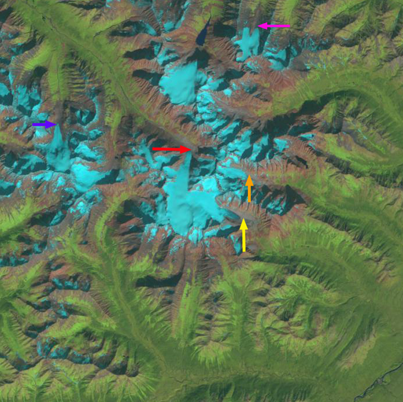
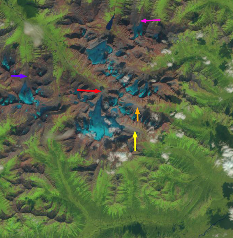
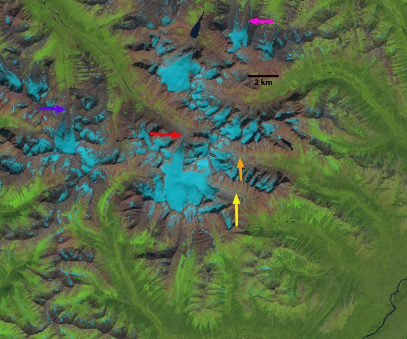
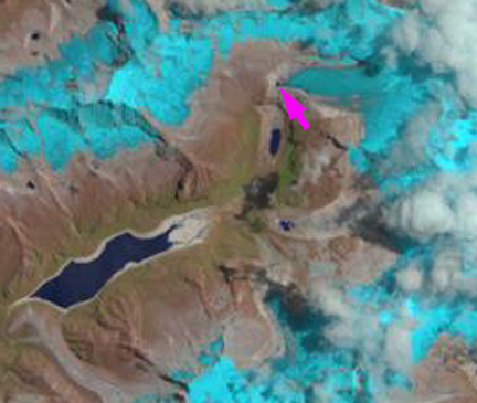
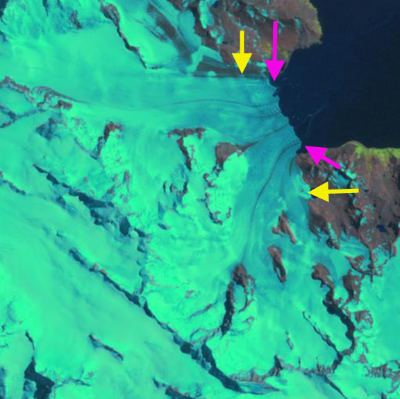
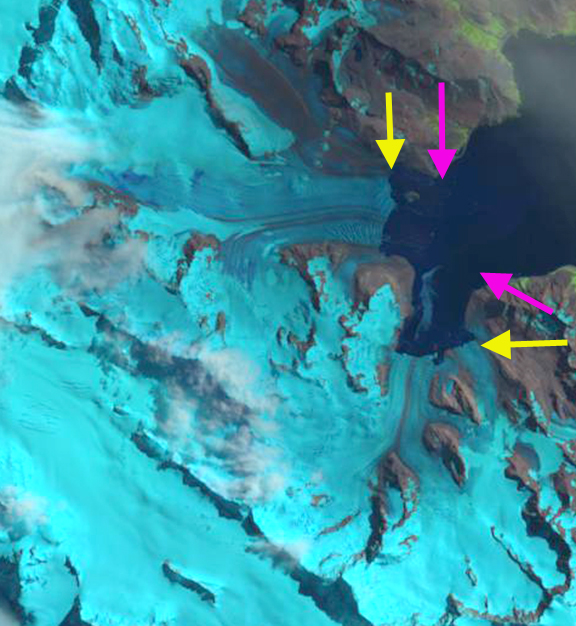
Gepatschferner Retreat 2012-2013-2014. Image from Austrian Alpine Club annual terminus survey report, Andrea Fischer.

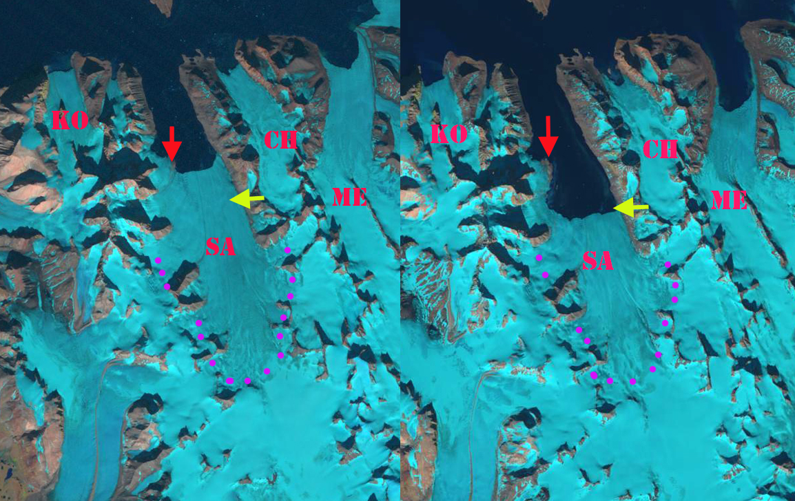
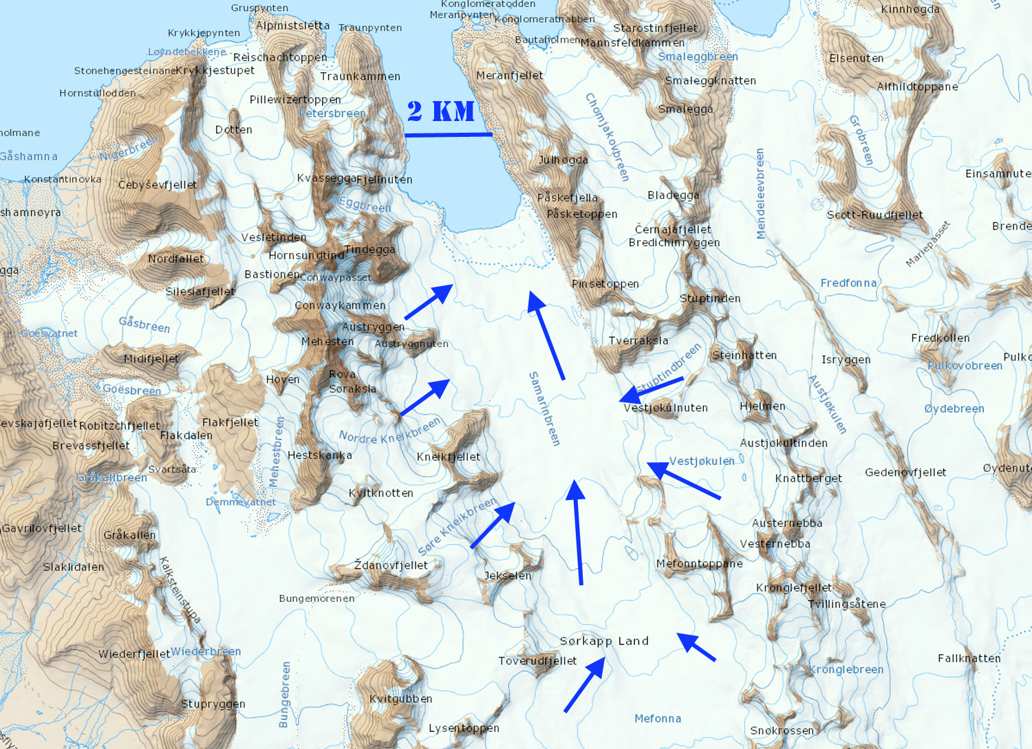
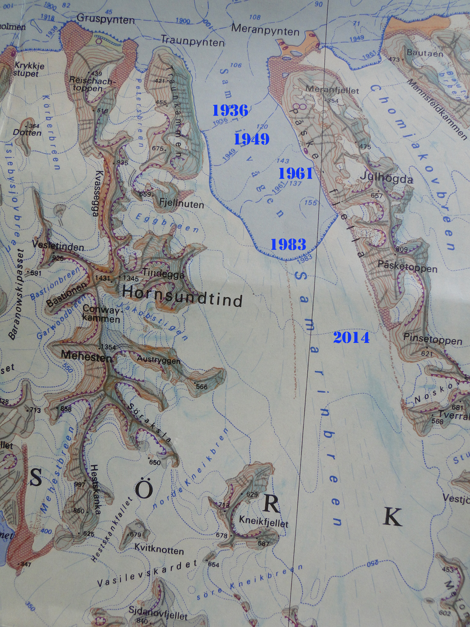
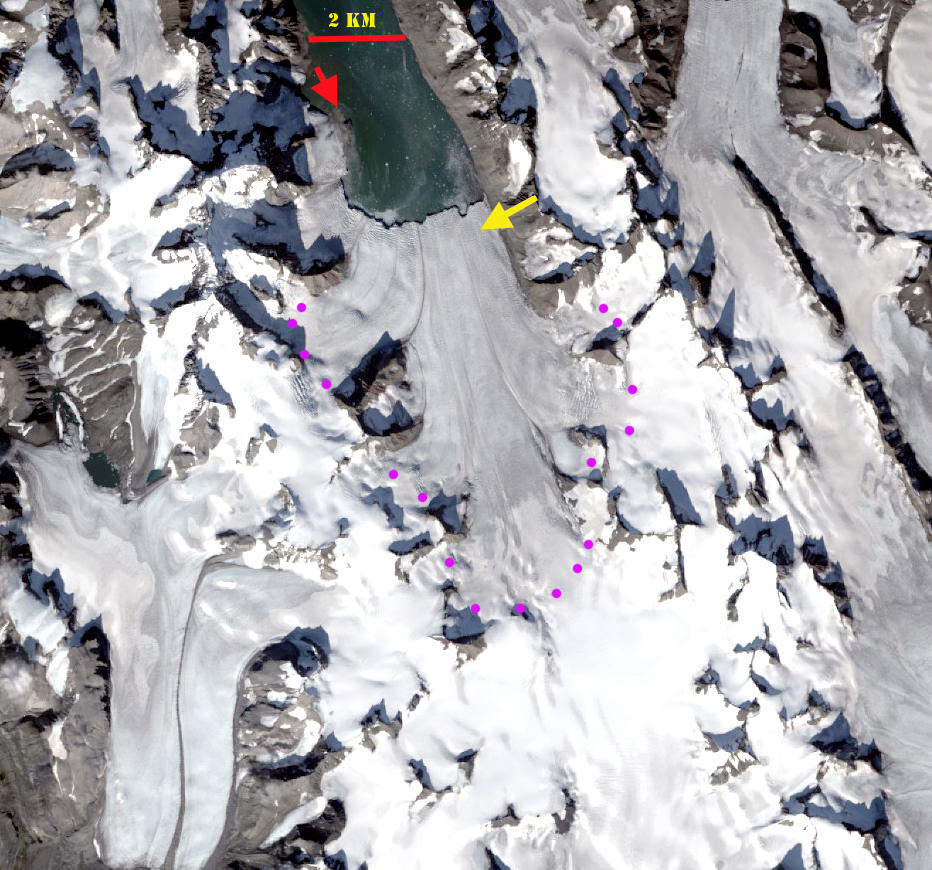
In Norway terminus fluctuation data from 38 glaciers for 2014 with ongoing assessment indicate, 33 retreating, and 3 were stable. The average terminus change was -12.5 m (Elverhoi, 2014). Mass balance surveys with completed results are available for seven glaciers; all have negative mass balances with an average loss exceeding -1063 mm. In 2014 Norway experienced its warmest year (NOAA, 2015). In Iceland the mass balance of Hofsjokull was -970 mm. Svalbard was a location of positive mass balance with all four glaciers having a small positive mass balance.

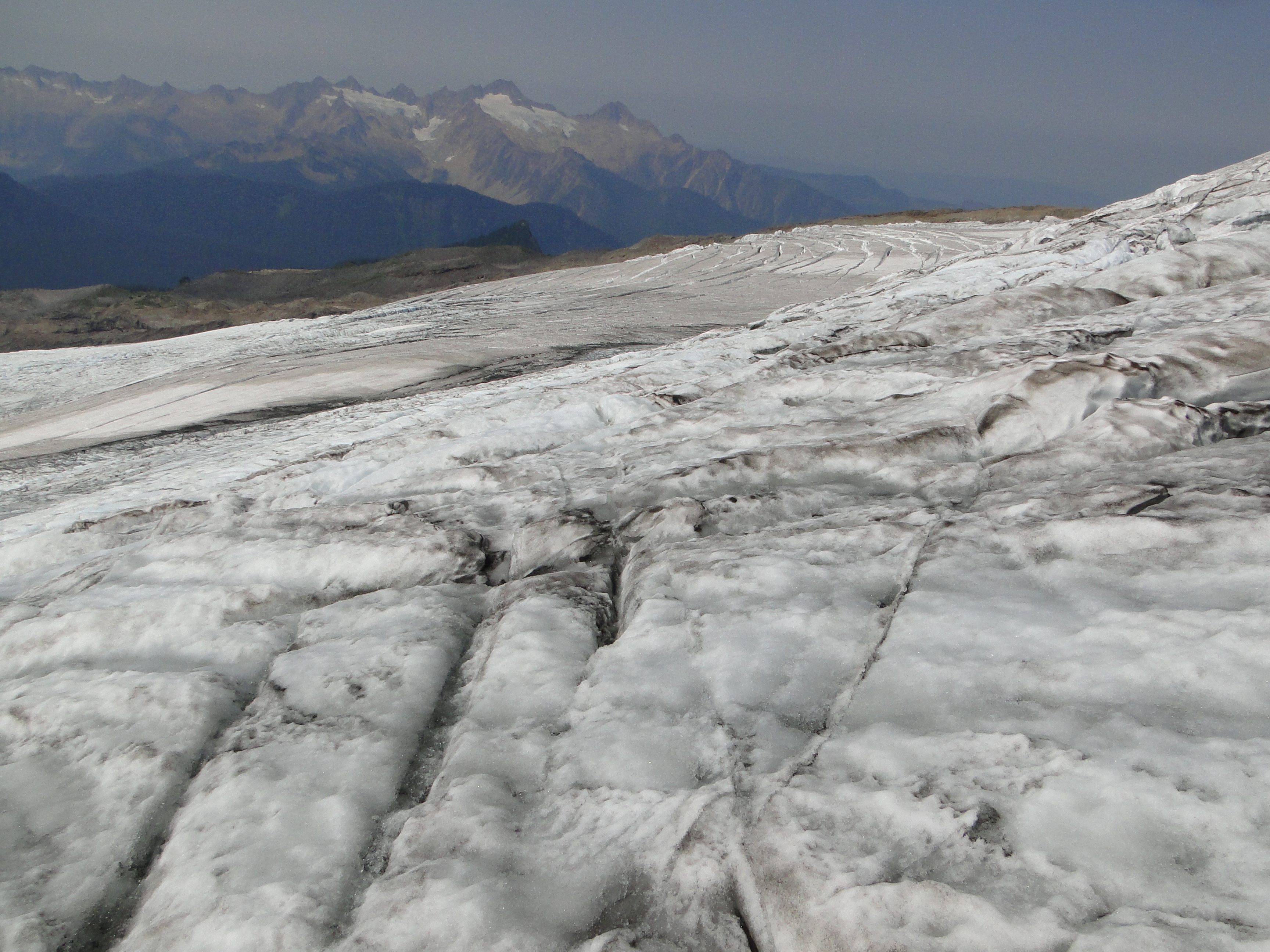
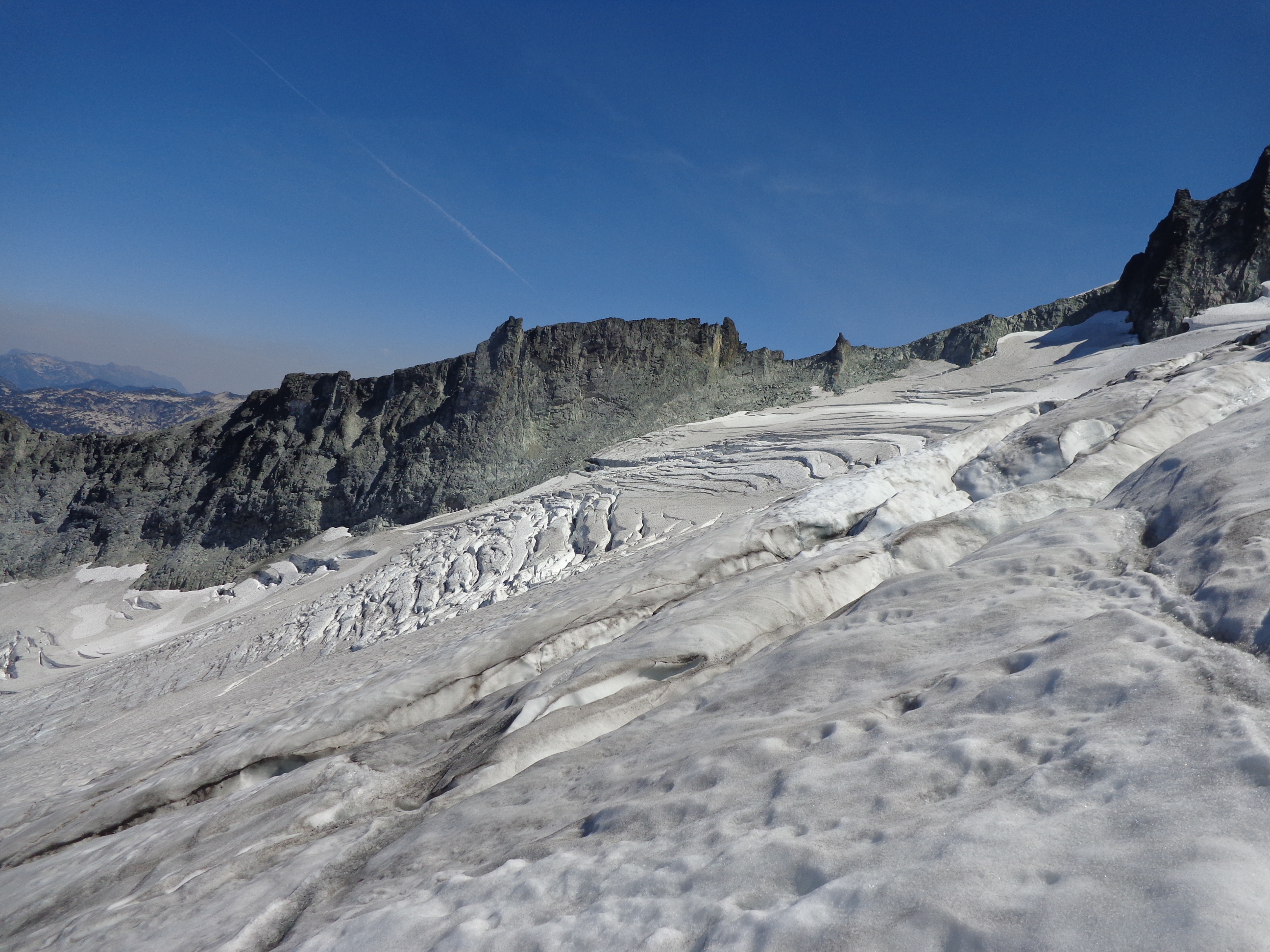
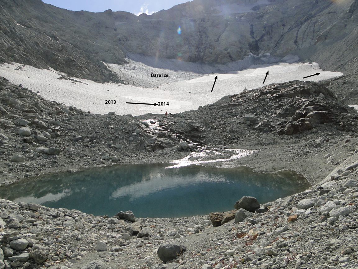
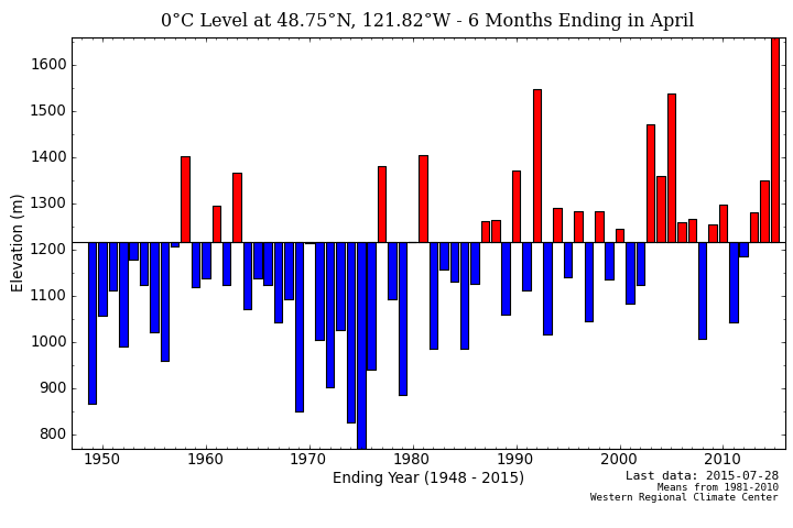
In Washington and Alaska mass balance data from 13 glaciers indicate a loss of -1185 mm. In Washington the melt season was exceptional with the mean June-September temperature tied with the highest for the 1989-2014 period and had the highest average minimum daily temperatures. The result in the North Cascade Range, Washington was a significant negative balance on all nine glaciers observed, with an average of -1000 mm w.e. and, unsurprisingly, all experienced retreat. In Alaska all three glaciers with mass balance assessed had significant negative mass balances.

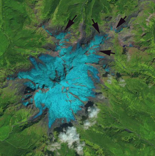
Lemon Creek Glacier, Alaska in 2014. Note the lack of snowpack in early September. The accumulation area ratio is 10 % coverage, and 62% coverage is needed for equilibrium. Picture taken by Chris McNeil

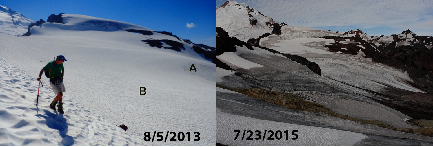
Rainbow Glacier September 2015, lack of snowcover again evident.

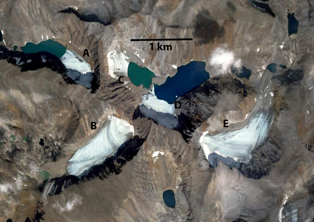
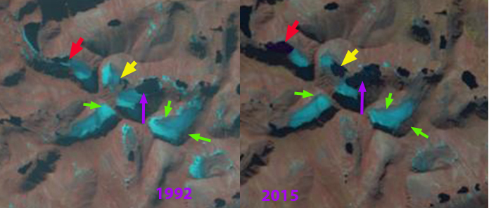
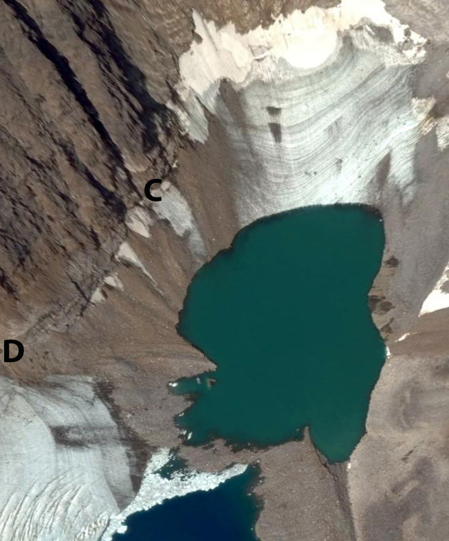
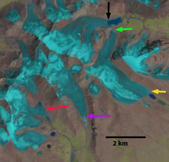
In the high mountains of central Asia five glaciers from four nations reported data were negative with a mean of -870 mm. Gardelle et al (2013) noted that mean mass balance in the eastern and central Himalaya was -275 mma^-1 and losses in the western Himalaya were 450 mma^-1 during the last decade.

References

Carturan, L., Baroni, C., Becker, M., Bellin, A., Cainelli, O., Carton, A., Casarotto, C., Dalla Fontana, G., Godio, A., Martinelli, T., Salvatore, M. C., and Seppi, R. 2013: Decay of a long-term monitored glacier: Careser Glacier (Ortles-Cevedale, European Alps). The Cryosphere, 7, 1819-1838, doi:10.5194/tc-7-1819-2013.

Elverhoi, H., 2014: Norwegian water resources and energy directorate 2013 glacier length change Table. http://www.nve.no/en/Water/Hydrology/Glaciers/

Fischer, A. 2013: Gletscherbericht 2012/2013. http://www.alpenverein.at/portal/news/aktuelle_news/2015/2015_04_03_gletscherbericht.php

Gardelle, J., Berthier, E., Arnaud, Y., and Kääb, A.: Corrigendum to “Region-wide glacier mass balances over the Pamir-Karakoram-Himalaya during 1999–2011” published in The Cryosphere, 7, 1263–1286, 2013, The Cryosphere, 7, 1885-1886, doi:10.5194/tc-7-1885-2013, 2013.

Haeberli, W., J. Cihlar and R. Barry 2000: Glacier monitoring within the Global Climate Observing System. Ann. Glaciol, 31, 241-246.

NOAA, 2015: State of the Climate: Global Analysis-2014: http://www.ncdc.noaa.gov/sotc/global/.

Pelto, M. 2010: Forecasting temperate alpine glacier survival from accumulation zone observations. The Cryosphere, 4, 67–75.

Pfeffer, W.T., and the Randolph Consortium 2014: The Randolph Glacier Inventory: a globally complete inventory of glaciers, J. Glaciol., 60 (221), 537-551 (doi: 10.3189/2014JoG13J176)

Radic´ V, Bliss A, Beedlow AC, Hock R, Miles E and Cogley JG (2014) Regional and global projections of twenty-first century glacier mass changes in response to climate scenarios from global climate models. Climate Dyn., 42(1–2), 37–58 (doi: 10.1007/s00382-013-1719-7)

Schaner, N., Voisin, N., Nijssen, B. and Lettenmaier, D. 2012: The Contribution of Glacier Melt to Streamflow. Environmental Research Letters 7 (doi:10.1088/1748-9326/7/3/034029.

WGMS, 2013: Glacier Mass Balance Bulletin No. 12 (2010–2011). Zemp, M., Nussbaumer, S. U., GärtnerRoer, I., Hoelzle, M., Paul, F., and Haeberli, W. (eds.), ICSU(WDS)/IUGG(IACS)/UNEP/UNESCO/WMO, World Glacier Monitoring Service, Zurich, Switzerland.

WGMS, 2015: Latest Glacier Mass Balance data. http://www.geo.uzh.ch/microsite/wgms/mbb/sum13.html

Samarinbreen, Svalbard Rapid Retreat 1990-2014

On July 15, 2015May 2, 2024 By mspeltoIn glacier climate change, Glacier Observations, svalbard glacier retreat

Samarinbreen (SA) 1990 left, and 2014 right, Landsat image comparison. KO=Korberbreen, CH=Chomjakovbreen,
ME=Mendeleevbreen Red arrows indicate 1990 terminus position, yellow arrows 2014 terminus. and purple dots the snowline.

Samarinbreen terminated in a calving front in Samarinvagan, a bay on the southern side of Hornsund Fjord. Hornsund is a fjord that in 2015 almost cuts through the southern Island of Svalbard, due to the retreat of Hamberbergbreen and Hornbreen. The Institute of Geophysics Polish Academy have maintained a Polish Research Station in Hornsund since 1957. The 1984 map, from the University of Silesia, of the glaciers and geomorphology document the extent of the glaciers in 1983 in the region. Blaszczyk et al (2009) analysis identified 163 Svalbard glaciers that are tidewater with the total length calving ice−cliffs at 860 km for the 2001-2006 period. They observed that 14 glaciers had retreated from the ocean to the land over the last 3-4 decades. Nuth et al (2013) determined that the glacier area over the entire archipelago has decreased by an average of 80 km2/year over the past 30 years, a 7% reduction.In the most recent period 1990-2007, terminus retreat was larger than in an earlier period from 1930-1990, while area shrinkage was smaller. A more detailed examination by the same researchers, Blaszczyk, Jania and Kolondra (2013) reported the total area of the glacier cover lost in Hornsund Fjord area from 1899–2010 was approximately 172 km2. The average glacier area retreat increased from a mean of 1.6 square kilometers per year to 3 square kilometers per year since 2000. Samarinbreen begins near the height of land of Sorkappland sharing the divide with Olsokbreen at an elevation of below 400 m.

Map from Topo Svalbard
Samarinbreen retreat is documented by the map produced by the University of Silesia; 1936-1949 retreat equals 750 m, 1949-1961 retreat equals 1200 m, 1961-1983 retreat equals 1700 m. Landsat imagery from 1990-2014 illustrates that the retreat of the glacier has been 2.1 km. The 1990 terminus is indicated by the red arrow, and the 2014 terminus is the yellow arrow. The tidewater front shows limited icebergs from calving in all images I have reviewed, yet calving must be a key means of volume loss. The snowline in 1990 is between 300 m in 1900. In 2014 the image is earlier in the melt season, but is at at 275 m. The 2012 image of the terminus region illustrates the snowline again near 300 m. There is limited glacier area above 400 m, indicating the high snowfall and low melt rate of the region allowing a glacier to have such a low mean elevation. That the snowline is consistently so close in elevation to the highest section of the glacier indicates that mass loss will continue as will retreat.

University of Silesia Map of Hornsund

Samrinbreen 2012 image from Topo Svalbard, red arrow indicates new island.

Russell Glacier, Greenland Rapid Snowline Rise K-Transect 2015

On July 10, 2015May 2, 2024 By mspeltoIn glacier climate change, Glacier Observations, Greenland glacier retreat2 Comments

Landsat Image based Watson River discharge sequence June 14-July 8, 2015

It was 30 years ago I first participated in Greenland Ice Sheet research, there was not much of it at the time. However, there was the recognition of the importance for sea level rise with global warming, and this was driving an increase in research at that time. The level of research has increased exponentially in the last decade. One long standing and remarkable program that indicates the long term thinking that has helped us develop an understanding of ice sheet changes, is the K-Transect of ablation stakes emplaced in the Russell Glacier Catchment. Here we examine the changing snowline from Mid-June to early July of 2015, as well as the longer term record. The Institute for Marine and Atmospheric Research Utrecht has maintained the best long term field based ablation record on the GIS, the K-Transect. This resulted in van de Wal et al., (2012) reporting on 21 years of surface mass balance in the region. At one site, S9 (1520 m) near the equilibrium line altitude (ELA), the long term record indicates a rise in the ELA in recent years, see figure below, and a more negative surface mass balance. This record has also been crucial in helping to build surface mass balance models for the GIS. The results updated daily from one such model, is at the Polar Portal, maintatined by the DMI – Danish Meteorological Institute, GEUS – The Geological Survey of Denmark and Greenland and DTU Space – National Space Institute. This summer the Automatic Weather Station on this transect Kan M, at 1270 m did not experience temperatures above 0 C until June 19th and they have been consistently above that since, (PROMICE, 2015). At S9 temperatures have been reaching 4 C most days in July (IMAU, 2015).

So Thank You to PROMICE, Polar Portal, IMAU, NASA and others for the remarkable progress and sharing of data.

K-Transect map from van As et al (2012)

Surface mass balance at S9 on the K-Transect from van de Wal (2012).
Supraglacial lakes were mapped in detail for the period by Fitzpatrick et al (2014), who found the lakes were forming several weeks earlier in 2010-2012 and at higher elevations than before. They also observed as seen in graph below that Watson River except for in 2010 had a distinct rise in flow in mid-July. Notice the lag between initial melt that fills lakes, volume loss shown, and the rise in Watson River.

Watson River discharge and lake volume loss in K-Transect region from Fitzpatrick et al (2014)

This all played out in the last few weeks. The melt season was off to a slow start in 2015 as indicated both by the Polar Portal and Landsat imagery, note on June 14th that lakes beyond the GIS had ice cover still, the snowline was at 750 m, blue dots, with spotty snow patches below this. The lack of melt in also evident in the lack of supraglacial lakes. Note the lack of discharge in Watson River, pink arrow. By June 29th melt had begun in earnest with the snowline moving inland 25 kilometers and rising to 1150 m. Discharge was greater, but still limited in Watson River. The main belt of supraglacial lakes, red arrow was at m. By July 8th, the snowline had moved more than 50 km inland since June 14th to an altitude of 1450 m. This is close to S9. The snowline is not the ELA on the GIS as there are zones of superimposed ice below the snowline. However, with the transient snowline this high in early July, the ELA will inevitably be higher than S9 at 1520 m. The discharge in Watson River will continue to rise and become more variable as the glacial hydorologic system matures van As et al (2012). This post will be updated with imagery from later in the 2015 ablation season.

Surface Mass Balance from model data

June 14, 2015 Landsat Image

June 29, 2015 Landsat Image
<a href="http:/
July 8, 2015 Landsat Image

Google Earth image showing late summer discharge of Watson RIver.

Share this:
Facebook
LinkedIn
X
Like Loading...

Big Four Glacier & Ice Caves, WA: a short future?

On July 8, 2015May 2, 2024 By mspeltoIn glacier climate change, Glacier Observations, North Cascade Glaciers

The Big Four ice caves area popular hiking destination 90 minutes northeast of Seattle in the North Cascades. This ice mass is currently the lowest elevation glacier in the lower 48 states. It is fed by tremendous avalanching from higher on Big Four Mountain. During the winter the snow piles up on the avalanche fan. In the summer the waterfall from above carves tunnels under the snow-ice mass. At some point in June or July the tunnels are enlarged enough to allow people, but also warm air to enter. This leads to further tunnel expansion. In warm summers the tunnels get large enough by late summer that collapses of the roof occur. Unfortunately this year the caves are already in late summer form and an expected collapse tragically led to the 1 person killed and five injured this week. Here we examine the formation and now demise of this odd glacier in the last decade. There are no pictures of the ice caves in this post, as it is not a place to enter this year.

The 1999-2002 period featured heavy winter snowpack and avalanching boosting Big Four. The summer of 2003 was the first of three cruel seasons to Big Four. In this image you cannot note the blue case to all but the very top of the avalanche cone, indicating it is older snow. There is further two layers that look to be annual layers on the right side of the image. This suggests to me, the base is a 1999, layer, than a 2000 layer, than a broader dirty band and a 2002 layer, followed by a 2003 snowpack,. The summer of 2001 was warm and no snowpack would have survived, causing the wider dirt band. In 2003-2005 a series of dismal winters and warm summers led to the near total loss of the Big Four Avalanche fan, at this point it was not a glacier.

From 2006-2012 a series of good summers led to redevelopment, which prompted David Head to contact me to investigate in 2009 if it was a glacier. He provided a series of images from 2005-2008 indicating the changes. We then headed to the glacier in 2009 to investigate in detail. In 2009 we mapped the glacier, from above and below. We found it had an area of 0.07 square kilometers, the glacier had a center length of 370 m, had a width at the toe of 270 m, an average slope of 22 degrees an average depth of 32 m a maximum depth of 55 m, and a volume of ~2 million cubic meters. There was blue glacier ice evident and a few crevasses on the upper portion. It was a glacier. The glacier gained at least 30 m in thickness over the majority of its area from 2005-2008, which is an extraordinarily short period. This year for the first time no avalanches reached the avalanche fan. Last summer was at record warmth, with the snowmass ablated to its smallest extent since 2005. The ice cave entrances were wide with a rainbow shaped arch, not an engineering setup for stability. This did not change over the winter. Hence, it is like having two summers in a row without winter. Contrast the June 2008 image to April 2015 (from Kellbell), quite a difference. There is no snow on Big Four even in April this year, the blue glacier ice is exposed and ablating starting then. The ice mass is rapidly ablating in the warm early summer of 2015 and will reach its smallest size since 2005 by the end of the summer. It is likely too thick to melt it all this year, but it may well surpass the 2005 minimum size. It will no longer be a glacier by the end of the summer. That is unusual to watch a glacier form and melt away in a decade. There will be more collapses in the ice caves this summer as it recedes to a meager size.

2003-2007 Time lapse of Big Four

June 2008 image

October 2008 image

August 2009 image

April 2015 (Kellbell)

Share this:
Facebook
LinkedIn
X
Like Loading...

Posts navigation

Older posts
Newer posts