2016 Field Season Results-North Cascade Glacier Climate Project

On October 14, 2016October 14, 2016 By mspeltoIn climate change glacier retreat, Glacier Observations, glaciers salmon

For Mount Baker, Washington the freezing level from January-April 20 was not as high as the record from 2015, but still was 400 m above the long term mean. April 1 snowpack at the key long term sites in the North Cascades was 8% above average. A warm spring altered this, with April being the warmest on record. The three-four weeks ahead of normal on June 10th, but three weeks behind 2015 record melt. The year was poised to be better than last year, but still bad for the glaciers. Fortunately summer turned out to be cooler, and ablation lagged. Average June-August temperatures were 0.5 F above the 1984-2016 mean and 3 F below the 2015 mean. The end result of our 33rd annual field season assessing glacier mass balance in the North Cascades quantifies this. Our Nooksack Indian Tribe partners again installed a weather and stream discharge station below Sholes Glacier.

The primary field team consisted of myself, 33rd year, Jill Pelto, grad student UMaine for the 8th year, Megan Pelto, Chicago based illustrator 2nd year, and Andrew Hollyday, Middlebury College. We were joined by Tom Hammond, NCCC President 13th year, Pete Durr, Mount Baker Ski Patrol, Taryn Black, UW grad student and Oliver Grah Nooksack Indian Tribe. The weather during the field season Aug. 1-17th was comparatively cool.

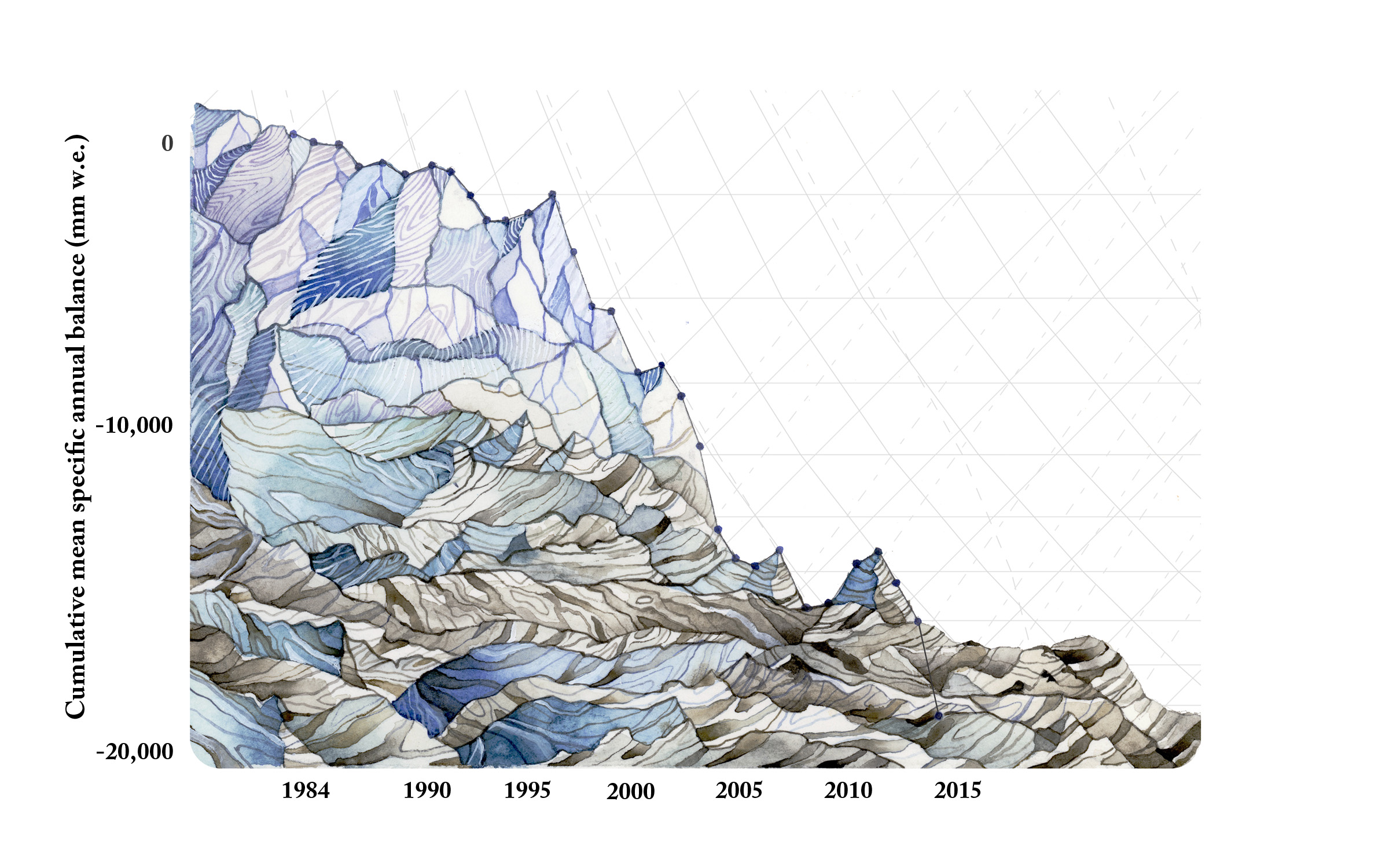
Mass Balance: Easton Glacier provides the greatest elevation range of observations. On Aug 2, 2016 the mean snow depth ranged from 0.75 m w.e. at 1800 m to 1.5 m w.e. at 2200 m and 3.0 m w.e. at 2500 m. Typically the gradient of snowpack increase is less than this. There was a sharp rise in accumulation above 2300 m. This is the result of the high freezing levels. The mass balances observed fit the pattern of a warm but wet winter. The high freezing levels left the lowest elevation glaciers Lower Curtis and Columbia Glacier with the most negative mass balance of approximately 1.5 m. The other six glaciers had negative balances of -0.6 to -1.2 m. This following on the losses of the last three years has left the glaciers with a net thinning of 6 m, which on glaciers averaging close to 50 m is a 12% volume loss in four years. We anticipate with that this winter will be cooler and next summer the glaciers happier. We will back to determine this.

Snowpack loss from Aug. 5-Sept. 22 is evident in the pictures below on Sholes Glacier. Detailed snow depth probing, 112 measurements, of the glacier on August 5th allows determination of ablation as the transient snow line traverses probing locations from Aug. 5. GPS locations were recorded along the edge of blue ice on each of the dates. Ablation during this period was 2.15 m.

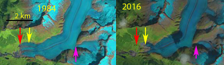
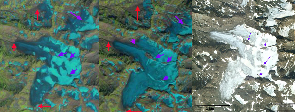
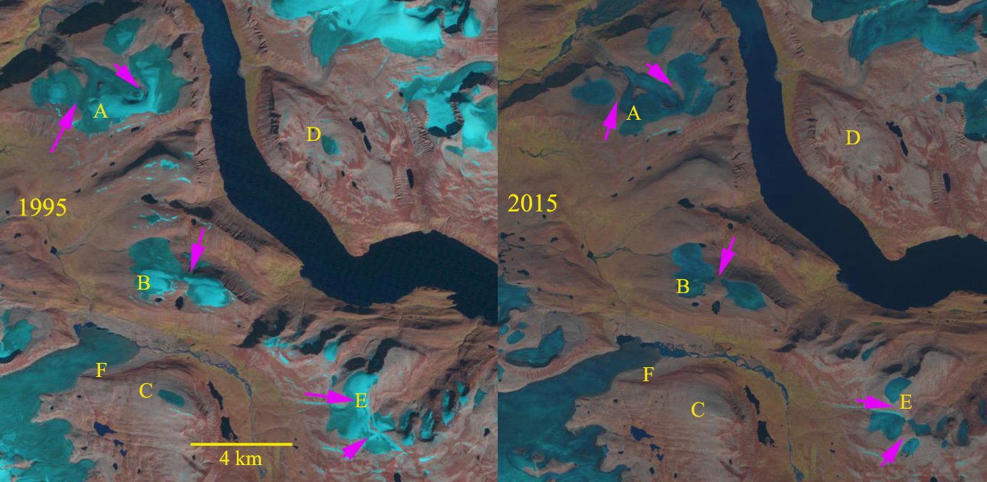
Terminus Change: We measured terminus change at several glaciers and found that a combination of the 2015 record mass balance loss and early loss of snowcover from glacier snouts in 2016 led to considerable retreat since August 2015. The retreat was 25 m on Easton Glacier, 20 m on Columbia Glacier, 20 m on Daniels Glacier, Sholes Glacier 28 m, Rainbow Glacier 15 m, Lower Curtis Glacier 15 m. The main change at Lower Curtis Glacier was the vertical thinning, in 2014 the terminus was 41 m high, in 2016 the terminus seracs were 27 m high. The area loss of the glaciers will continue to lead to reduced glacier runoff. We continued to monitor daily flow below Sholes Glacier which allowed us to determine that in August 2016 45% of the flow of North Fork Nooksack River came from glacier runoff. This is turns has impacts for the late summer and fall salmon runs.

South Sawyer Glacier Retreat and Separation, Alaska

On September 20, 2016May 2, 2024 By mspeltoIn alaska glacier retreat, climate change glacier retreat, glacier climate change, Glacier Observations1 Comment

Comparison of South Sawyer Terminus position and unnamed glacier just to the south. Red arrows are the 1985 terminus and yellow arrows the 2016 position of each terminus.

South Sawyer Glacier is a 50 km long tidewater glacier terminating at the head of Tracy Arm fjord in Southeast Alaska. The winding fjord surrounded by steep mountains is fed by Sawyer and South Sawyer Glacier is home to stellar sea lions, humpback whales and harbor seals. This combination makes it attractive for cruise ships. Mike Greenfelder a Naturalist/Photography Instructor with Lindblad Expeditions suggested I examine this glacier, and he provided several images. I had a chance to observe the glacier in 1982 and 1984 and noted that the snowline of the glacier at 1125 meters by Pelto (1987), using Landsat images. We also identified the water depth at the glacier front was 180-200 m and the velocity of the calving front in the 1980’s was 1800 m/year (Pelto and Warren, 1990). Today the velocity had declined to less than half of this, which is expected given that water depth at the front in the most recent charts from 1999 indicate 1985 terminus position water depth is 110 m (Elliot et al, 2012). This is deep but not as deep as in the 1980’s, the greater the water depth, the greater the degree of buoyancy at the front and the higher the calving rate. The glacier retreated 3.5 km from 1899-1967 and then experienced little retreat from 1967 to 1985 (Molnia et al, 2008). Larsen et al (2007) observed a rapid thinning of the Stikine Icefield during the 1948-2000 period.The retreat has been driven by rising snowlines in the region that has driven the retreat of North Dawes, Baird, Dawes and Sawyer Glacier. Here we use Landsat images to indicate from 1985-2016 to identify terminus change and recent snowline elevation.

The terminus has retreated 2300 m from 1985 to 2016, with little retreat from 1985 to 1996. Of equal importance is the glacier now appears to be near the tidewater limit of Tracy Arm. In the gallery of terminus images below from Mike Greenfelder, the 2005 and 2012 images illustrate a sharp increase in slope at Point B and red arrows in 2015 just the red arrows, 300 m from the ice front. In 2016 the ice front is nearly to the base of this icefall. This represents a sharp rise in the bed of glacier causing an icefall. Whether the bed is entirely above sea level is not clear. Just south of the main terminus is a separate glacier that in 1985 was the combination of two tributaries. By 2016 the two glaciers have separated with a retreat of 4.5 km for the western arm and 3.8 km for the eastern arm.

In the gallery of snowline images it is evident that upglacier there are two tributaries that joined the main glacier in 1985, that no longer reach the glacier in 2016. This is indicative of the higher snowlines and thinning glacier. The gallery of snowlines indicate the last date during the melt season with clear imagery of the snowline. In 1985 the snowline was at 1250 m, in 1996 the snowline was at 1400 m, in 2013 1400 m, in 2014 1600 m, in 2015 at 1400 m and in 2016 at 1650 m. The images are close to the end of the melt season, but are a minimum elevation for the equilibrium line. The snowline is averaging 300 m higher than it did in the 1980’s. The retreat of South Sawyer Glacier and its iceberg production will slow as the water depth at the front declines in the near future. The retreat will continue due to the sharp rise in snowlines that has occurred which has led to significant thinning up to 1500 m noted by Larsen et al (2007). The retreat of neighboring non-calving glaciers emphasizes this point.

[ngg_images source=”galleries” container_ids=”27″ display_type=”photocrati-nextgen_basic_imagebrowser” ajax_pagination=”1″ template=”/nas/wp/www/sites/blogsorg/wp-content/plugins/nextgen-gallery/products/photocrati_nextgen/modules/ngglegacy/view/imagebrowser-caption.php” order_by=”sortorder” order_direction=”ASC” returns=”included” maximum_entity_count=”500″]

Herbert Glacier Retreat, Alaska 1984-2016

On September 14, 2016May 2, 2024 By mspeltoIn alaska glacier retreat, climate change glacier retreat1 Comment

Comparison of Herbert Glacier terminus position in Landsat images from 1984 and 2016. Red arrow 1984 terminus, yellow arrow 2016 terminus and pink arrow a tributary that has separated.

Herbert Glacier drains the west side of the 4000 square kilometer Juneau Icefield in Southeast Alaska. It is the glacier just north of the more well known Mendenhall Glacier and just south of Eagle Glacier. It is also the first glacier I ever visited, July 3, 1981 during my first field season with the Juneau Icefield Research Program. Here we examine the changes from the August 17, 1984 Landsat 5 image to a Sept. 1, 2016 Landsat 8 image.

The glacier descended out of the mountains ending on the coastal plain in 1948. In 1984 we examined the terminus of this glacier, which was in the small proglacial lake at 150 m. Herbert Glacier has retreated 600 m since 1984. The width of the terminus has also declined. The pink arrow indicates a tributary that no longer feeds the main glacier. The retreat has not been enhanced by iceberg calving as is the case at Mendenhall Glacier. The overall retreat is also less than Eagle Glacier. In the Google Earth images below from 2005 and 2013 the retreat is 200 m, the terminus has fewer crevasses in 2013 suggesting a reduced velocity and faster retreat to come. The annual equilibrium line on the glacier has averaged 1150 m from 2003-2016. By contrast in August 1984 I skied to the top of the icefall and could see the snowline was at 1000 m. This leaves the glacier with an AAR of 0.45, too low to sustain equilibrium, retreat will continue. In 2015 and 2016 the snowline rose to over 1400 m by the end of the melt season, indicating two years of large mass loss, which will drive further retreat. The higher snow line elevation has been observed across the icefield Pelto et al (2013).

Transient snow line in Early Sept. of 2015 and 2016. The snow line is at the top of the icefalls, at 1400-1450 m.

2005 Google Earth Image, red line is 2005 margin, yellow line is 2013.

2005 Google Earth Image, red line is 1984 margin, yellow line is 2005.

Herbert Glacier Terminus in 2012

World Glacier Monitoring Service 30th Anniversary

On September 8, 2016May 2, 2024 By mspeltoIn climate change glacier retreat, glacier climate change, Glacier Observations

The numbers on the left y-axis depict quantities of glacial mass loss from the WGMS and sea level rise, and the suns across the horizon contain numbers that represent the global increase in temperature, coinciding with the timeline on the lower x-axis From Jill Pelto

The World Glacier Monitoring Service (WGMS) celebrated 30 years of achievement last week. I have had the privilege of being the United States representative to the WGMS and was an invited speaker for the Jubilee held in Zurich, Switzerland along with Matthias Huss, Wilfried Haeberli, Liss Marie Andreassen and Irene Kopelman. This post examines the important role that WGMS has and continues to serve under the leadership of Michael Zemp. The organization has been compiling, homogenizing and publishing data on glacier fluctuations and mass balance primarily from 1986-2013. WGMS remains the leading organization for the collection, storage and dissemination of information on the fluctuations of alpine glaciers. The resulting standardized collection of alpine glacier data that is archived by WGMS, is also leading to analysis efforts that otherwise would be hampered by limited data and lack of homogeneity to the data. Glaciers are recognized as one of the best climate indicators. Mass balance data is the best parameter to measure on glaciers for identifying climate change, because of its annual resolution. The core of the WGMS data set has been frontal variations, which indicate longer response to climate as well as dynamic changes. The key data set today provided by WGMS are the reference glaciers.

This set of glaciers has a 30-year continuous record of annual mass balance measured in the field, and each glacier also has geodetic verification. This mass balance data set is featured on the Global Climate Dashboard at NOAA. I report the mass balance of two reference glaciers Lemon Creek Glacier in Alaska and Columbia Glacier in Washington. Today the field based work is being increasingly supplemented and supplanted by remote sensing methods. This data sets indicates a period of sustained mass balance loss, and glacier retreat that Zemp et al (2015) using WGMS data noted as historically unprecedented. The most recent compilation publication is the Global Glacier Change Bulletin.

This data set is of particular value during this period of climate change and is already chronicling the disapperance of a number of glaciers in the data set. Glacier loss is not a process that has been well documented. The WGMS data set can be enriched by more data from expanding monitoring, reporting data from archives and simply adding the submission of data as a step in the research process for those monitoring alpine glaciers. The video of my presentation looking at 33 consecutive years of field work and sharing this data after compilation with the WGMS is below. The slides below are from the Jubilee presentations.

[ngg_images source=”galleries” container_ids=”32″ display_type=”photocrati-nextgen_basic_imagebrowser” ajax_pagination=”1″ template=”/nas/wp/www/sites/blogsorg/wp-content/plugins/nextgen-gallery/products/photocrati_nextgen/modules/ngglegacy/view/imagebrowser-caption.php” order_by=”sortorder” order_direction=”ASC” returns=”included” maximum_entity_count=”500″]

Kronotsky Peninsula, Kamchatka Glacier Fragmentation/Retreat

On August 25, 2016May 2, 2024 By mspeltoIn climate change glacier retreat, russia glacier retreat

The Kronotsky Peninsula is on the east coast of Kamchatka and has an small concentration of alpine glaciers. A recent paper by Lynch et al (2016) indicates a significant recession during the start of the 21st century in Kamchatka. They note a 24% loss in area, leading to fragmentation and an increase in the number of ice masses that could be considered glaciers. Lynch et al (2016) further note that the primary climate change has been a recent significant rise in summer temperature. It is interesting how few and small the glaciers are in Kamchatka versus similar latitudes of Alaska.

The red arrows indicate the 2000 terminus position. Purple arrows indicate areas of bedrock expansion within the 2000 glacier region. Google Earth image is same 2013 image.

A comparison of 2000 and 2015 Landsat images indicates the retreat of several glaciers and the expansion of bedrock glaciers within the previous accumulation zone areas. The snowcovered area in Sept. of 2000 is 35%, in Sept. 2015 the snowcovered area is 15%. Summer temperature anomalies for Kamchatka have been high in June and July of 2016 (NOAA, 2016). The result is that in August, 2016 despite the cloud cover it is evident that snowcover is less than 10% with time left in the melt season. September is one of the least cloudy months and if better imagery becomes available I will update this image here. The elevation of the glaciers is 2400-3700 m, relatively high. The termini of all three glaciers have retreated 200-400 m, which given the short time span and small size of the glaciers is significant. The lack of retained snowcover in recent years indicates that these glaciers lack a persistent accumulation zone and cannot survive (Pelto, 2010). A closeup of the terminus of the glaciers indicate all have low slopes, limited crevassing, and are poised more further retreat. Of the three termini the southern one indicates a recsssional moraine set (R). The western glacier concentric crevasses that indicate subsidence of terminus area (C). The northern glacier has significant supraglacial stream channels that took multiple years to develop, indicative of limited development (B).

2016 Landsat image of Krontosky Peninsula Glaciers

[ngg_images source=”galleries” container_ids=”34″ display_type=”photocrati-nextgen_basic_imagebrowser” ajax_pagination=”1″ template=”/nas/wp/www/sites/blogsorg/wp-content/plugins/nextgen-gallery/products/photocrati_nextgen/modules/ngglegacy/view/imagebrowser-caption.php” order_by=”sortorder” order_direction=”ASC” returns=”included” maximum_entity_count=”500″]

Glaciers in BAMS State of Climate 2015

On August 2, 2016May 2, 2024 By mspeltoIn climate change glacier retreat, glacier climate change, Glacier Observations

Decrease in Glacier Mass Balance uses measurements from 1980-2014 of the average mass balance for a group of North Cascade, WA glaciers. Mass balance is the annual budget for the glaciers: total snow accumulation minus total snow ablation. Not only are mass balances consistently negative, they are also continually decreasing. Glaciers have been one of the key and most iconic examples of the impact of global warming.

BAMS State of Climate 2015 asked me about featuring some of the glacier images for the cover, and I countered with a suggestion to utilize one of a series of paintings by Jill Pelto that illustrate the impact of climate change magnifying the impact of the data. Below are sections of this years report that focus on glaciers.

Glaciers and ice caps (outside Greenland)

M. Sharp, G. Wolken, L.M Andreassen, A. Arendt, D. Burgess, J.G. Cogley, L. Copland, J. Kohler, S. O’Neel, M. Pelto, L.Thompson, and B. Wouters

Among the seven glaciers for which 2014-2015 annual mass balance have been reported, the mass balances of glaciers in Alaska and Svalbard (three each) were negative, while the balance for Engabreen Glacier in Norway was positive. The pattern of negative balances in Alaska and Svalbard is also captured in time series of regional total stored water estimates, derived using GRACE satellite gravimetry, which are a proxy for regional total mass balance (ΔM) for the heavily glacierized regions of the Arctic (Figure 3). Measurements of ΔM in 2014-2015 for all the glaciers and ice caps in Arctic Canada and the Russian Arctic also show a negative mass balance year. The GRACE-derived time series clearly show a continuation of negative trends in ΔM for all measured regions in the Arctic. These measurements of mass balance and ΔM are consistent with anomalously warm (up to +1.5ºC) summer air temperatures over Alaska, Arctic Canada, the Russian Arctic, and Svalbard in 2015, and anomalously cool temperatures in northern Scandinavia, particularly in early summer (up to -2ºC). The warmer temperatures led to higher snowlines in the aforementioned regions as seen in images below.

Baffin Island Ice Cap near Clephane Bay indicate limited snowpack in 2015

Frostisen Ice Cap, Svalbard with limited 2015 snowpack.

Alpine Glaciers

M.Pelto

Preliminary data for 2015 from 16 nations with more than one reporting glacier from Argentina, Austria, Canada, Chile, Italy, Kyrgyzstan, Norway, Switzerland, and United States indicate that 2015 will be the 32nd consecutive year of negative annual balances with a mean loss of -1169 mm for 33 reporting reference glaciers and -1481 mm for all 59 reporting glaciers. The number of reporting reference glaciers is 90% of the total whereas only 50% of all glaciers that will report have submitted data thusfar. The 2015 mass balance will likely be comparable to 2003, the most negative year at -1268 mm for reference glaciers and -1198 mm for all glaciers.

The cumulative mass balance loss from 1980-2015 is 18.8 m, the equivalent of cutting a 20.5 m thick slice off the top of the average glacier (Figure 1). The trend is remarkably consistent from region to region (WGMS, 2015). The decadal mean annual mass balance was -261 mm in the 1980’s, -386 mm in the 1990’s, –727 mm for 2000’s and -818 mm from 2010-2015. The declining mass balance trend during a period of retreat indicates alpine glaciers are not approaching equilibrium and retreat will continue to be the dominant terminus response (Zemp et al., 2015). The recent rapid retreat and prolonged negative balances has led to many glaciers disappearing and others fragmenting (Pelto, 2010; Carturan et al, 2015).

In South America seven glaciers in Columbia, Argentina and Chile reported mass balance. All seven glaciers had losses greater than 1200 mm, with a mean of -2200 mm. These Andes glaciers span 58 degrees of latitude.

In the European Alps, mass balance has been reported for 14 glaciers from Austria, France, Italy and Switzerland. All 14 had negative balances exceeding 1000 mm, with a mean of -1865 mm. This is an exceptionally negative mass balance rivaling 2003 when average losses exceeded -2000 mm.

In Norway mass balance was reported for six glaciers in 2015, all six were positive with a mean of 780 mm. This is the only region that had a positive balance for the year. In Svalbard six glaciers reported mass balances, with all six having a negative mass balance averaging -675 mm.

In Alberta, British Columbia, Washington and Alaska mass balance data from 17 glaciers was reported with a mean loss of -2590 mm, with all 17 being negative. This is the most negative mass balance for the region during the period of record. From Alaska south through British Columbia to Washington the accumulation season temperature was exceptional with the mean for November-April being the highest observed.

In the high mountains of central Asia six glaciers from Russia, Kazakhstan, and Kyrgyzstan reported data, all were negative with a mean of -660 mm.

Columbia Glacier having lost nearly all of its snowcover by early August had its most negative mass balance of any years since measurements began in 1984

Thirty-third Annual North Cascade Glacier Climate Project Field Season Underway

On July 31, 2016May 2, 2024 By mspeltoIn climate change glacier retreat, glacier climate change, Glacier Observations, glaciers salmon, North Cascade Glaciers4 Comments

Base Map of the region showing main study glaciers, produced by Ben Pelto.

From President Reagan to President Obama each August since 1984 I have headed to the North Cascade Range of Washington to measure the response of glaciers to climate change. Specifically we will measure the mass balance of nine glaciers, runoff from three glaciers and map the terminus change on 12 glaciers. The data is reported to the World Glacier Monitoring Service. Three glaciers that we have monitored annually have disappeared since 1984.

In 2016 for Mount Baker, Washington the freezing level from January-April was not as high as the record from 2015, but still was 400 m above the long term mean. The snowpack on June 1st was three weeks behind last year’s record melt, but still three to four weeks of head of normal. July has been exceptionally cool reducing this gap. With all the snow measurement stations losing snowcover by July 1, the gap is uncertain until we arrive on the glaciers. This will not be a good year, but will be a significant improvement over last year, likely more in the 2012 or 2013 category. Each location is accessed by backpacking in and camping in tents.

We will first travel north to Mount Baker and the Easton Glacier, we will be joined by Oliver Lazenby, Point Roberts Press. We will then circle to the north side where I expect we will be joined by Jezra Beaulieu and Oliver Grah, Nooksack Indian Tribe. Jen Lennon from the Sauk-Suiattle Tribe and Pete Durr, Mount Baker Ski Patrol are also planning to join us here. When we head into Columbia Glacier Taryn Black from U of Washington will join us. The field team consists of Mauri Pelto, 33^rd year, Jill Pelto, UMaine for the 8^th year, Megan Pelto, 2^nd year, and Andrew Hollyday, Middlebury College. Tom Hammond, 13^th year will join us for a selected period.

[ngg_images source=”galleries” container_ids=”38″ display_type=”photocrati-nextgen_basic_imagebrowser” ajax_pagination=”1″ template=”/nas/wp/www/sites/blogsorg/wp-content/plugins/nextgen-gallery/products/photocrati_nextgen/modules/ngglegacy/view/imagebrowser-caption.php” order_by=”sortorder” order_direction=”ASC” returns=”included” maximum_entity_count=”500″]

Aug.   1: Hike into Easton Glacier.
Aug.   2: Easton Glacier
Aug.   3: Easton Glacier
Aug. 4: Hike Out Easton Glacier, Hike in Ptarmigan Ridge
Aug.   5: Sholes Glacier
Aug.   6: Rainbow Glacier
Aug.   7: Sholes Glacier and/or Rainbow Glacier
Aug. 8: Hike out and into Lower Curtis Glacier
Aug. 9: Lower Curtis Glacier
Aug. 10: Hike out Lower Curtis Glacier- Hike in Blanca Lake Mail Pickup Maple Falls, WA 98266
Aug. 11: Hike in Columbia Glacier
Aug. 12: Columbia Glacier
Aug. 13: Hike out Columbia Glacier; Hike in Mount Daniels
Aug. 14: Daniels and Lynch Glacier
Aug. 15: Ice Worm Glacier
Aug. 16: Ice Worm Glacier, Hike out Mount Daniels-Hike out

Sater Glacier, Alaska Not Retaining Snowcover

On July 28, 2016May 2, 2024 By mspeltoIn alaska glacier retreat, climate change glacier retreat

2012 Google Earth Image. Purple arrows indicate areas where the margin is receding well above the lowest terminus.

Sater Glacier is in the Okpilak River watershed of the Brooks Range, Alaska. It is named for John Sater an early geologist working in the Brooks Range and on the nearby McCall Glacier. Here we examine Landsat imagery from 1987-2016 to identify changes in the glacier. Matt Nolan, U. Alaska-Fairbanks, has provided links to the recent research and publications at McCall Glacier. These glacier have suffered increased mass loss since 1990 as a result of an increase in the equilibrium line altitude that has reduced accumulation area and is indicative of increased ablation (Delcourt al , 2008) as noted at Slender Glacier.

In 1987 Sater Glacier extended from 2300 m to 1600 m with two main tributaries joining 1 km above the terminus. Retained snowcover blankets most of the glacier in this early August image. In 1995 the main change is the lack of retained snowcover on the glacier, with a month left in the melt season. The retained snowcover is the accumulation area ratio (AAR), which needs to be above 50% for a glacier to be in equilibrium, but is less than 10% in 1995. The 2012 Google Earth image above indicates very little retained snowcover on the glacier in mid-July, AAR of 15%. Likely no retained snowcover by summer’s end. In 2015 a late July image again indicates limited retained snowcover, the AAR less than 10%. In 2016 the late July image again indicates limited snowcover though slightly better than in 2015 with an AAR of 25%. This persistent failure to retain snowcover indicates a glacier than cannot survive (Pelto, 2010). This has also led to the near separation of the tributaries, retreat of the upper margins of the glacier and terminus retreat of 250 m. The retreat of the terminus has been much less than Okpilak Glacier, but the prognosis due to the lack of retained snowcover is much worse, it cannot survive current climate.

1987 Landsat image red arrow indicates 1987 terminus, yellow arrow 2015 terminus and purple arrows upglacier thinning.

1995 Landsat image red arrow indicates 1987 terminus, yellow arrow 2015 terminus and purple arrows upglacier thinning.

2015 Landsat image red arrow indicates 1987 terminus, yellow arrow 2015 terminus and purple arrows upglacier thinning.

2016 Landsat image red arrow indicates 1987 terminus, yellow arrow 2015 terminus and purple arrows upglacier thinning.

Sjögren Glacier Fast Flow, Fast Retreat, Antarctica

On July 21, 2016May 2, 2024 By mspeltoIn Antarctic Glacier retreat, climate change glacier retreat, glacier climate change1 Comment

Sjögren Glacier comparison in Landsat images from 2001 and 2016, red dots indicate terminus position, Point A, B, C and D are in fixed locations.

Sjögren Glacier flows east from the northern Antarctic Peninsula and prior to the 1980’s was a principal feeder glacier to Prince Gustav Ice Shelf. This 1600 square kilometer ice shelf disintegrated in the mid-1990’s and was gone in 1995 (Cook and Vaughan, 2010). Scambos et al (2014) noted a widespread thinning and retreat of Northern Antarctic Peninsula Glaciers with the greatest changes where ice shelf collapse had occurred, Sjögren Glacier being one of the locations. Scambos et al (2004) first documented the acceleration of glaciers that fed an ice shelf after ice shelf loss in the Larsen B region. A new paper by Seehaus et al (2016) focuses on long term velocity change at Sjögren Glacier as it continues to retreat. This study illustrates the acceleration is long lived with a peak velocity of 2.8 m/day in 2007 declining to 1.4 m/day in 2014, compared to a 1996 velocity of 0.7 m/day, which was likely already higher than the velocity in years prior to ice shelf breakup. Here we examine Landsat images from 1990, 2001, 2005 and 2016 to illustrate changes in terminus position of Sjögren Glacier

In the 1990 Landsat image Sjögren Glacier feed directly into the Prince Gustav ice Shelf which then By 1993 Seehaus et al (2016) note that Sjögren Glacier had retreated to the mouth of Sjögren Inlet in 1993, this is marked Point A on Landsat Images. By 2001 the glacier had retreated to Point B, a distance of 7 km. Between 2001 and 2005 Sjögren Glacier retreat led to a separation from Boydell Glacier at Point C. In 2016 Sjögren Glacier had retreated 10-11 km from the 2001 location, and 4.5 km from Point C up the expanding fjord. The production of icebergs remains heavy and the inlet does not narrow for another 6 km from the front. Seehaus et al (2016) Figure 1 indicates that the area of high velocity over 1 m/day extends 1 km upglacier, with somewhat of a slowdown at 6 km behind the front. The high velocity and limited change in fjord width in the lower 6 km indicates there is not a new pinning point to slow retreat appreciably in this stretch. Figure 1 also illustrates the retreat from 1993-2014. The pattern of ice shelf loss and glacier retreat after loss has also played out at Jones Ice Shelf and Rohss Bay.

1990 Landsat Image of Sjogren Glacier and Prince Gustav Ice Shelf, terminus marked by red dots

2005 Landsat Image of Sjogren Glacier, terminus marked by red dots

Chaupi Orko Glaciers, Bolivia Extensive Recession

On July 18, 2016May 2, 2024 By mspeltoIn bolivia glacier retreat, climate change glacier retreat

Landsat comparison of the Chaupi Orko Glaciers from 1988, 1999 and 2015. Red arrows indicate 1988 terminus and yellow arrows the 2015 terminus location.

Chaupi Orko is a 6044 m Andean peak in the Cordillera Apolobamba on the Peru-Bolivia border with glaciers radiating from it summit. Here we examine a pair of glaciers on the southern side of the mountain that drain into Laguna Suches, which is split by the Bolivia-Peru border. Laguna Suches is most known for placer gold mining. Glaciers in Bolivia have been experiencing substantial retreat during the last 40 years, such as at Nevada Cololo. The glaciers of the Apolobamba have lost 48% of their area from 1975-2006 (Hoffmann, 2012). Hoffmann and Weggenmann (2012) observed both the extensive retreat, new lake formation, and the potential problem of glacier lake outbursts in this region, which is part of the Apolobamba Integrated Natural Management Area. In a continuation of these studies an excellent study in review by Cook et al (2016) indicates a 43% decline in glacier area in the Cordillera Apolobamba from 1986 to 2014. They identified a total of 25 lakes with some risk of GLOF, though historic occurrences to date in the area are few. They further found an decrease in proglacial lakes in contact with glaciers during this period. The glaciers here are summer accumulation type with the ablation occurring during the dry season from May-October .

In 1988 the southwest Chaupi Orko Glacier (W), red arrow, does not have a proglacial lake at its terminus. The southern Chuapi Orko Glacier (S) ends adjacent to a small lake east of the terminus, red arrow. By 1999 a small proglacial lake has formed at the terminus of the southwest Chaupi Orko Glacier. The southern Chaupi Orko Glacier has receded 350 m. By 2015 the southwest Chaupi Orko Glacier has retreated to the yellow arrow, with the proglacial lake having expanded to an area of 0.35-0.4 square kilometers. Retreat of the west glacier has ranged from 500 to 800 m. The southern Chaupi Orko Glacier has retreated 600 m exposing two new small proglacial lakes that it has since largely retreated from. The lakes are narrow and too small to be a Glacier lake outburst flood (GLOF) threat. This particular basin does not pose a GLOF threat with no substantial lake below the south glacier and only the small, apparently shallow lake below the west glacier. A small island in the midst of the lake, suggests lake not very deep. The west glacier has a calving face enhancing retreat (IC).Neither glacier indicates significant thinning higher on the glacier, suggests limited melting. This is a region of significant ablation via sublimation vs melting, which is not as efficient a process for mass loss and is enhanced during La Nina periods (Vuille et al, 2008). The reduction of glacier area does lead to declines in glacier runoff, which will have a more widespread impact.

Small island amidst proglacial lake from the west glacier, also ice cliff noted.

Google Earth image of the Chaupi Orco region.

Conducting Long Term Annual Glacier Monitoring

On June 29, 2016May 2, 2024 By mspeltoIn climate change glacier retreat, glacier climate change, North Cascade Glaciers

Easton Glacier in 1990, 2003 and 2015 from same location. Below Painting by Jill Pelto of crevasse assessment using a camline.

This is the story of how you develop and conduct a long term glacier monitoring program. We have been monitoring the annual mass balance of Easton Glacier on Mount Baker, a stratovolcano in the North Cascade Range, Washington since 1990. This is one of nine glaciers we are continuing to monitor, seven of which have a 32 year long record. The initial exploration done in the pre-internet days required visiting libraries to look at topographic maps and buying a guide book to trails for the area. This was followed by actual letters, not much email then, to climbers who had explored the glacier in the past, for old photographs. Armed with photographs and maps we then determined where to locate base camp and how to access the glacier. The first year is always a test to make sure logistically you can reach enough of the glacier to actually complete the mass balance work with a sufficiently representative network of measurement sites. The second test is if you can stand the access hike, campsite, and glacier navigation, to do this every year for decades; if the answer is no, move on. That was the case on Boulder Glacier, also on Mount Baker: poor trail conditions and savage bugs, were the primary issue. Next we return to the glacier at the same time each year, completing the same measurements each year averaging 210 measurements of snow depth or snow melt annually. This occurs whether it is gorgeous and sunny, hot, cold, snowy, rainy, or recently on this glacier dealing with thunderstorms. You wake up, have your oatmeal and coffee/cider/tea, and get to work. Lunch on the snow features bagels, dried fruit, and trail mix. Happy hour features tang or hot chocolate depending on the weather. It is then couscous, rice, pasta or quinoa for dinner, with some added dried vegetable or avocado. The sun goes behind a mountain ridge and temperatures fall, and the tent is the haven until the sun returns. Repeat this 130 times on this glacier and you have a 25 year record. During this period the glacier has lost 16.1 m of water equivalent thickness, almost 18 m of thickness. For a glacier that averaged 70 m in thickness this is nearly 25% of the volume of the glacier gone. The glacier has not maintained sufficient snow cover at the end of the summer to have a positive balance, this is the accumulation area ratio, note below. The glacier has retreated 315 m from 1990-2015. This data is reported annually to the World Glacier Monitoring Service. The glacier has also slowed its movement as it has thinned, evidenced by a reduction in number of crevasses. During this time we have collaborated with researchers examining the ice worms, soil microbes/chemistry, and weather conditions on the ice. This glacier supplies runoff to Baker Lake and its associated hydropower projects. Our annual measurements here and on Rainbow Glacier and Lower Curtis Glacier in the same watershed provide a direct assessment of the contribution of glaciers to Baker Lake. The glacier is adjacent to Deming Glacier, which supplies water to Bellingham, WA. The Deming is too difficult to access, and we use the Easton Glacier to understand timing and magnitude of glacier runoff from Deming Glacier.

The glacier terminates at an elevation of 1650 m, but thinning and marginal retreat extends much higher. A few areas of bedrock have begun to emerge from beneath the ice as high as 2200 m. The changes in ice thickness are minor above 2500 m, indicating this glacier can retreat to a new equilibrium point with current climate.

Mass balance, terminus and supra glacial stream assessment are illustrated in the video, Filmed by Mauri Pelto, Jill Pelto, Melanie Gajewski, with music from Scott Powers.

Mass balance Map in 2010 of Easton Glacier used in the field for reference in following years.

Accumulation Area Ratio/Mass balance relationship for Easton Glacier

Chutanjima Glacier Retreat & High Snowline, Tibet, China 1991-2015

On June 21, 2016May 2, 2024 By mspeltoIn china glacier retreat, climate change glacier retreat, glacier climate change, Glacier Observations

A comparison of three Tibet glaciers in 1988, 1991 and 2015 Landsat images. Red arrows are the 1988 terminus position, yellow arrow the 2015 terminus location and purple dots the snowline in late October 2015. U=unnamed, CH=Chutanjima Glacier and MO=Mogunong Glacier: which did not retreat significantly and lacks a red arrow.

A recent European Space Agency Sentinel-2A image of southern Tibet, China and Sikkim illustrated three very similar glaciers extending north from the Himalayan divide on the China-India Border. We examine these three glacier in this post. The three glaciers all drain into the Pumqu River basin, which becomes the Arun River. The largest is unnamed the two easternmost are Chutanjima and Mogunong Glacier.The glaciers all have similar top elevations of 6100 -6200 m and terminus elevations of 5260-5280 m. All three are summer accumulation type glaciers with most of the snow accumulating during the summer monsoon, though this is also the dominant melt period on the lower glacier. Wang et al (2015) examined moraine dammed glacier lakes in Tibet and those that posed a hazard, none of the three here were identified as hazardous. The number of glacier lakes in the Pumqu Basin has increased from 199 to 254 since the 1970’s with less than 10% deemed dangerous, but that still leaves a substantial and growing number (Che et al, 2014). Here we compare Landsat images from 1988, 1992 and 2015 to identify their response to climate change. The second Chinese Glacier inventory (Wei et al. 2014) indicated a 21% loss in glacier area in this region from 1970 to 2009.The pattern of retreat and lake expansion is quite common as is evidenced by other area glaciers, such as Gelhaipuco, Thong Wuk, Baillang Glacier and Longbashaba Glacier.

In the 1988 image all three glaciers terminate at the southern end of a proglacial lake with seasonal lake ice cover, red arrows. In 1991 the lakes are ice free and have some icebergs in them. By 2015 the retreat has been 500 m for the easternmost glacier, 400 m for Chutanjima Glacier and 100 m at most for Mogunong Glacier. Each glacier has remained extensively crevassed to the terminus indicating they remain vigorous. The retreat is greatest for the two ending in expanding lakes. Mogunong Glacier appears to be near the upper limit of the lake, and is not calving, which likely led to less retreat. An icefall is apparent 700 m from the front of Mogunong Glacier. The width of the glacier below this point has diminished considerably from 1988 to 2015, though retreat has been minor, indicating a negative mass balance. There is an icefall 1 km from the icefront of Chutanjima, indicating the maximum length the lake would reach.

The Sentinel image indicates an important characteristic and trend in the region. This is an early February image and the snowline is quite high on the glacier in the midst of winter. The snowline is at 5850-5900 m nearly the same elevation as in late October of 2015 seen above. This illustrates the lack of winter accumulation that occurs on these summer accumulation glaciers. It also indicates a trend toward ablation processes remaining active, though limited from November-February. The lack of snowcover on the lower glaciers as the melt season begins hastens ablation zone thinning, mass balance loss and retreat.