Rio Engaño, Chile Headwater Glacier Retreat GLOF Threat Drops

On March 6, 2018April 28, 2024 By mspeltoIn chile glacier melt, chile glacier retreat, Glacier Observations

Comparison of glaciers at the headwaters of Rio Engaño in 1984 and 2018 Landsat images. The 1984 terminus location with red arrows, yellow arrows the 2018 terminus location, purple arrows wind drift patterns.

Rio Engaño drains into Lago General Carrera and its headwaters is a group of alpine glaciers. In March of 1977 one of the glaciers, generated a glacier lake outburst flood (GLOF) that reached a depth of 1.5 m at the small village of Bahía Murta Viejo 25 km down river (Anacona, et al 2015). Davies and Glasser (2012) observe that glaciers just northeast of the Northern Patagonia Icefield lost area at a rate of 0.2% per year from 1986-2011. Paul and Molg (2014) observed a more rapid retreat of 25% total area lost from glaciers in northern Patagonia from 1985-2011, the study area was north of the Northern Patagonia Icefield, including the Cordillera Lago General Carrera icefield.

Here we examine changes of four glaciers at the headwaters of Rio Engaño using Landsat imagery for the 1984 to 2018 period.

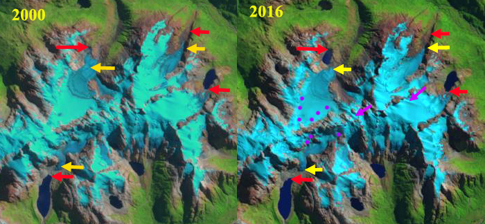
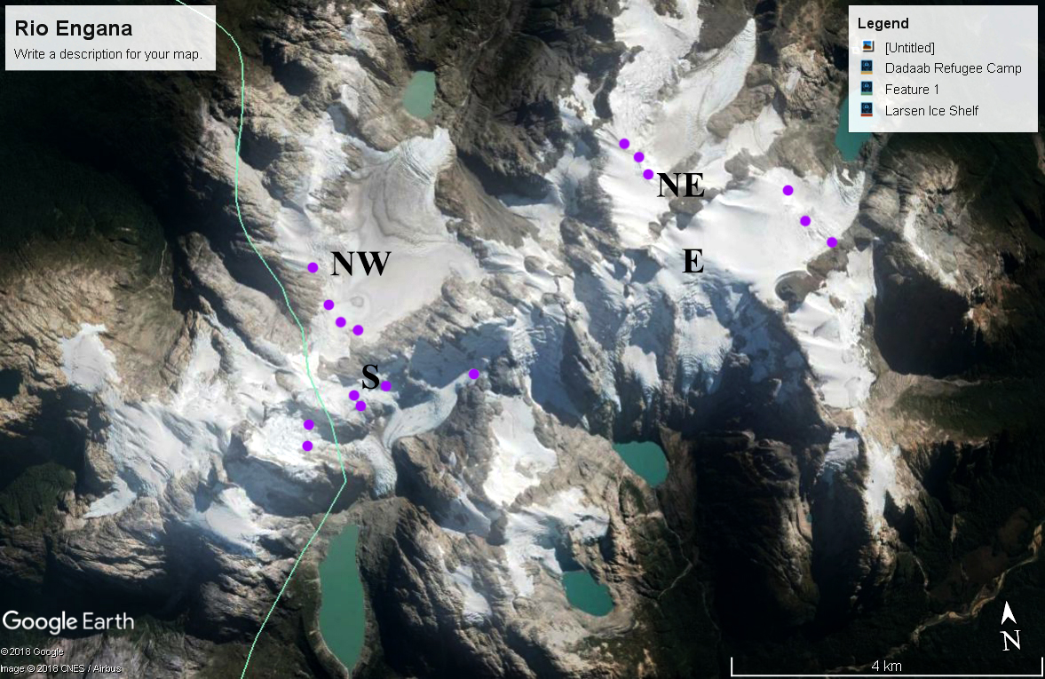
In 1984 the Northwest (NW) glacier had two terminus tongues and no lake at the terminus, red arrow. The Northeast (NE) glacier had a length of 4 km. The East (E) glacier terminated at the margin of a proglacial lake. The South (S) Glacier which experienced the GLOF, terminated on the northern end of a proglacial lake. By 2000 the NW glacier had lost its eastern terminus and a small lake is forming at the western terminus. The NE glacier had retreated 400 m. The S glacier no longer reaches the proglacial lake. In 2016 the snowline is quite high on the NW and S glacier, purple dots. The wind features, purple arrow indicate the strong wind sculpted features from the west winds. In 2018 the NW glacier no longer reaches the proglacial lake that began forming after 1984, total retreat 800 m. The NE Glacier has retreated 700 m and is now 3.3 km long. The E glacier terminates at the base of a steep slope 200 m from the proglacial lake it reached in 1984. The S glacier has retreated 600 m from the lake it reached in 1984. The NE and E glacier have substantial areas above 1600 m and have retained snowpack each year over a significant portion of the glacier. The NW and S glaciers have little area above 1600 m and in several years have retained minimal snowpack and will continue a rapid retreat.

Wilson et al (2018) documented a 43% increase in the number of glacial lakes and 7% in the area of lakes in the central and Patagonian Andes. In the Rio Engaño headwaters both the area and number of lakes has increased. The threat of GLOF in for these specific glaciers appears to be declining as the glaciers retreat further from the lakes. Iribarren et al (2014) list that glacier contact and glacier steepness adjacent to the lake are variables that raise GLOF hazards, and these factors are declining at the Rio Engaño headwaters. They also noted that the GLOF in 1977 had a volume of 7.36 million cubic meters the second largest in their record of 16 GLOF’s.

Comparison of glaciers at the headwaters of Rio Engaño in 2000 and 2016 Landsat images. The 1984 terminus location with red arrows, yellow arrows the 2018 terminus location, purple arrows wind drift patterns and purple dots the snowline in 2016.

Google Earth image from 2017 indicating the snowline leaving limited snowcovered area on NW and S glacier.

Gora Gvandra Glaciers, Caucasus Mountains, No Accumulation Zone in 2017

On February 15, 2018April 28, 2024 By mspeltoIn Caucasus Glacier retreat, Glacier Observations

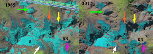
Comparison of glaciers around Gora Gvandra, Caucasus Mountians in 1985 and 2017 Landsat images. G=Gvandra Glacier, D=Dalar galcier, DN =North Dalari Glacier, S=Sakeni Glacier and M=Morde Glacier.

Gora Gvandra Mountain is southwest of Mount Elbrus of the Caucasus Mountains of Georgia and is surrounded by a group of glaciers that in recent years have not exhibited an accumulation zone. Stokes et al (2006) note that 94% of Caucasus Mountain glaciers retreated from 1985 to 2000. Tielidze and Wheate (2018) updated these observations to 2014 documenting the 1986 glacier surface area at 1482 square kilometers decreasing to 1193 square kilometers by 2014, a 29% decline. Here we examine Landsat images from 1985 to 2017 to illustrate the profound changes. In 2017 five of the six glaciers in the area had no retained snowpack, like the Alps this was a summer of high melt.

A comparison from 1985 to 2017 of Dalari North Glacier (DN), pink arrow indicates the glacier ending in a lake in 1985 and 1998, and terminates short of the lake in 2013. In 2013 the accumulation zone is small and in 2017 the accumulation zone does not exist. Note the contraction of the unnamed glacier from 1985-2017 at the green arrow, with an expanding bedrock area in the midst of what was the glacier and no retained snow in 2017. The Morde Glacier (M) terminus separated around a bedrock knob at the orange arrow in 1985 and the western arm terminates beyond the knob. The glacier has retreated 400 m by 2017, driven by a the lack of an accumulation zone with no retained snowpack in 2013 or 2017. The terminus of Dalar Galcier (D), yellow arrow, is below a steep slope in 1985 and 1998. By 2013 the steep slope is bare rock separating the former terminus from the rest of the glacier. In 2017 there is no retained snowpack on the glacier. Gvandra Glacier has lost all of its snowpack in 2017. The Sakeni Glacier has a 500 m wide terminus tongue in 1985 and 1998, white arrow. By 2013 and in 2017 the tongue has narrowed to 150 m and is going to either separate from the upper glacier or melt away soon. There is retained snowpack on the upper part of Sakeni Glacier in each year.

Of the six glaciers examined only one glacier had an accumulation zone in 2017 and in 2013 the accumulation zone was only significant on one glacier. Pelto (2010) noted that a glacier cannot survive without a persistent and consistent accumulation zone. This has been noted to be case even on some larger glacier of Mount Elbrus. Psysh Glacier in the western Caucasus is also disappearing.

Comparison of glaciers around Gora Gvandra, Caucasus Mountians in 1985 and 2017 Landsat images. yellow arrow=Dalar glacier, pink arrow=North Dalari Glacier, whtie arrow=Sakeni Glacier and orange arrow=Morde Glacier.

From a Glaciologists Perspective AGU Day 3

On December 14, 2017April 28, 2024 By mspeltoIn glacier climate change, Glacier Observations

Snapshot of day 3 of Glaciology poster presentations at AGU. The amount of glaciology research is impressive, there is much we do not know. We can no longer say that we know very little about any aspect or region. Before saying that explore the vast literature that is now available.

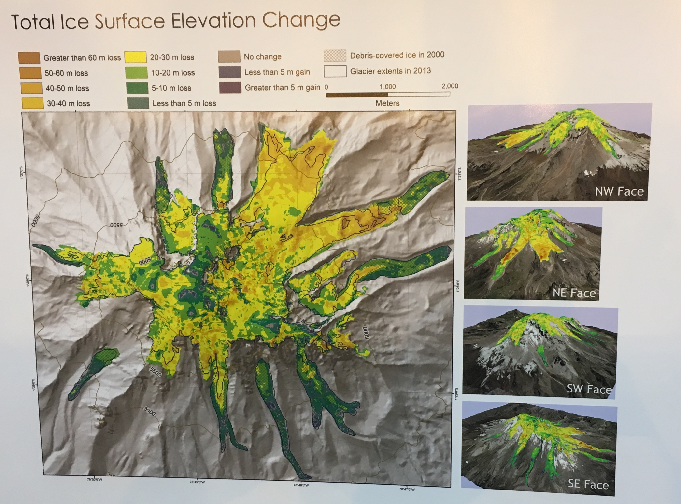
Jeff La Freniere at Gustavus Adolphus College used several new technologies, aerial and terrestrial LIDAR and structure-from-motion photogrammetry from drones make mass balance measurements using geodetic approaches increasingly feasible in remote mountain locations like Volcán Chimborazo, Ecuador. The result combined with a unique, 5-meter resolution digital elevation model derived from 1997 aerial imagery, reveal the magnitude and spatial patterns of mass balance behavior over the past two decades. Above are the results they found more specifically that on the Hans Meyer Glacier terminus, the mean surface elevation change since 1997 has been nearly 3 m yr^-1, while on the lower-elevation Reschreiter Glacier the mean elevation change has been approximately 1 m yr^{-1 .}

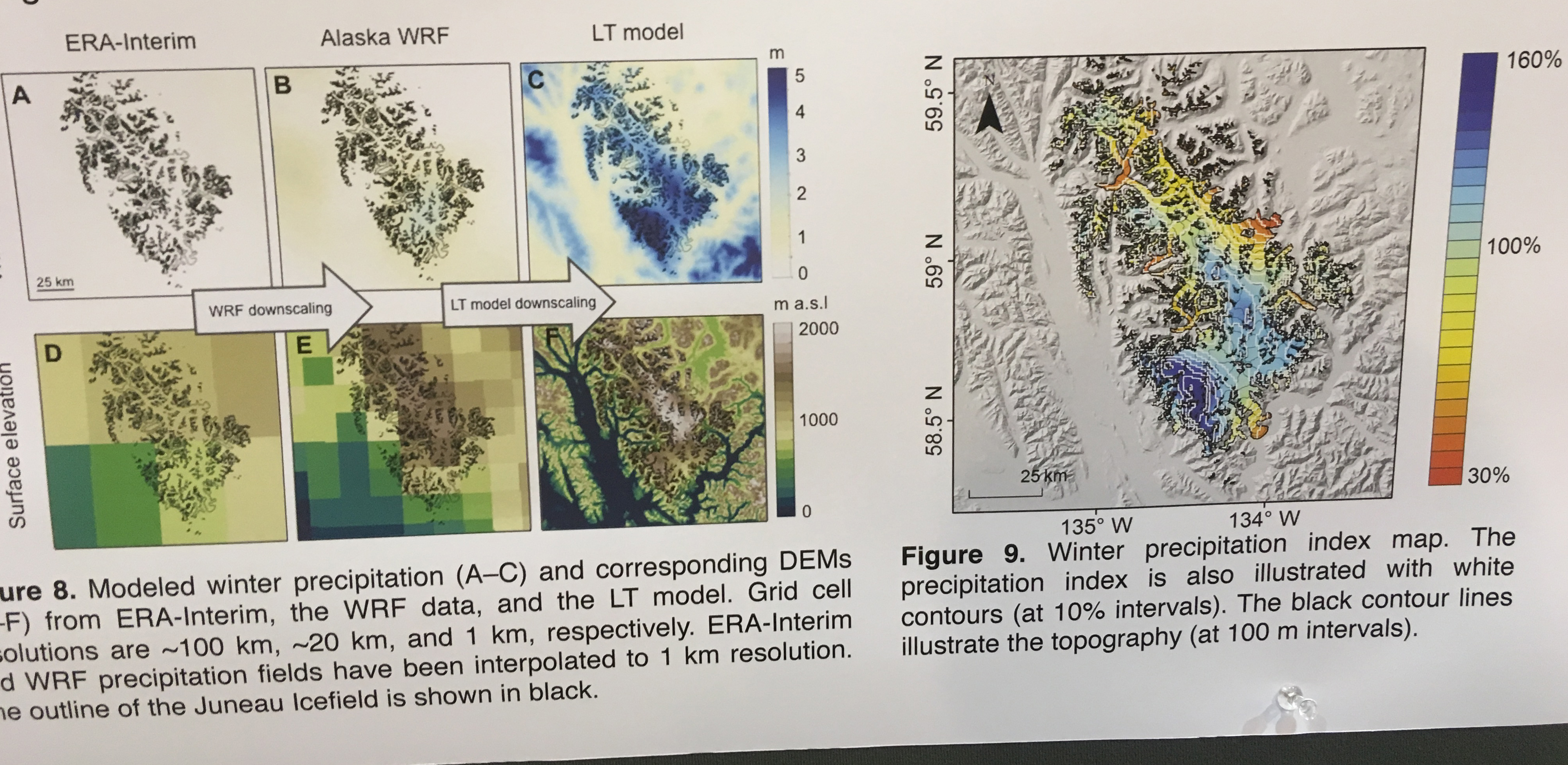
Aurora Roth, University of Alaska Fairbanks developed and applied a linear theory of orographic precipitation model to downscale precipitation to the Juneau Icefield region over the period 1979-2013. This LT model is a unique parameterization that requires knowing the snow fall speed and rain fall speed as tuning parameters to calculate cloud time delay. The downscaled precipitation pattern produced by the LT model captures the orographic precipitation pattern absent from the coarse resolution WRF and ERA-Interim precipitation fields. Key glaciological observations were used to calibrate the LT model. The results of the reference run showed reasonable agreement with the available glaciological measurements, which is what glacier mass balance observations have shown. The precipitation pattern produced was consistent regardless of horizontal resolution, and climate input data, but the precipitation amount varied strongly with these factors. The import is to help model mass loss from glaciers in Southeast Alaska which will alter downstream ecological systems as runoff patterns change.

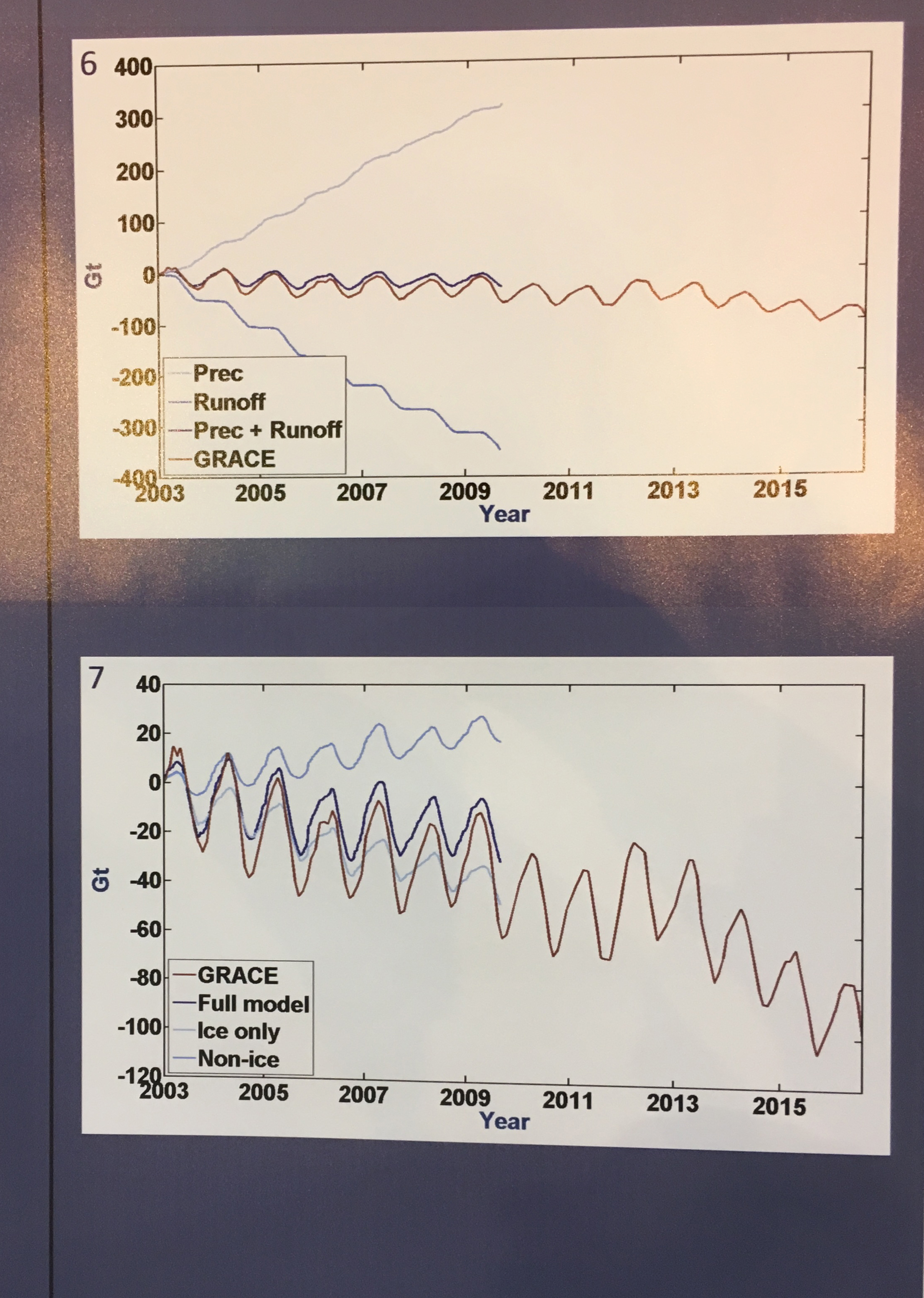
Joanna Young, University of Alaska Fairbanks focuses on partitioning GRACE glacier mass changes from terrestrial water storage changes both seasonally and in long-term trends using the Juneau Icefield, which has long term glacier mass balance data, as a case study for . They leverage the modeling tool SnowModel to generate a time series of mass changes using assimilated field observations and airborne laser altimetry, and compare to GRACE solution from the NASA Goddard Space Flight Center Geodesy Laboratory . This is one of the first to analyze GRACE at the sub-mountain range scale, and to examine terrestrial water storage trends at a smaller scale than the full Gulf of Alaska. The figure above looks at subannual and long-term changes of the Juneau Icefield from 2003 to present.

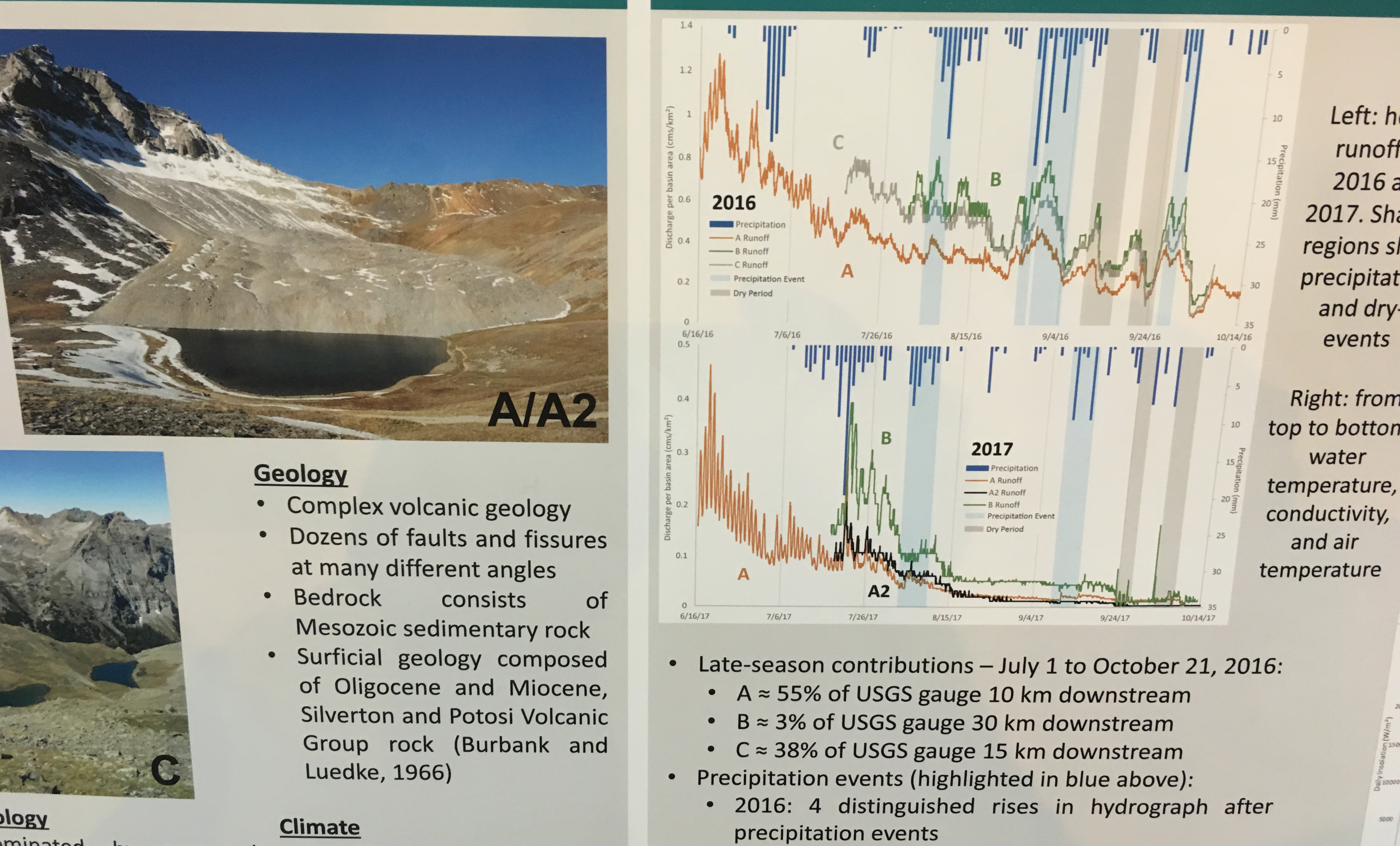
Emilio Ian Mateo, University of Denver Looked at rock glaciers in the San Juan Mountains of Colorado examining how slope aspect and rising air temperatures influenced the hydrological processes of streams below rock glaciers. Detailed findings illustrated above from 2016 and 2017 show that air temperature significantly influenced stream discharge below each rock glacier. Discharge and air temperature patterns indicate an air temperature threshold during late summer when rock glacier melt increased at a greater rate. The results suggest that slope aspect influences stream discharge, but temperature and precipitation are likely the most components of the melt regimes.

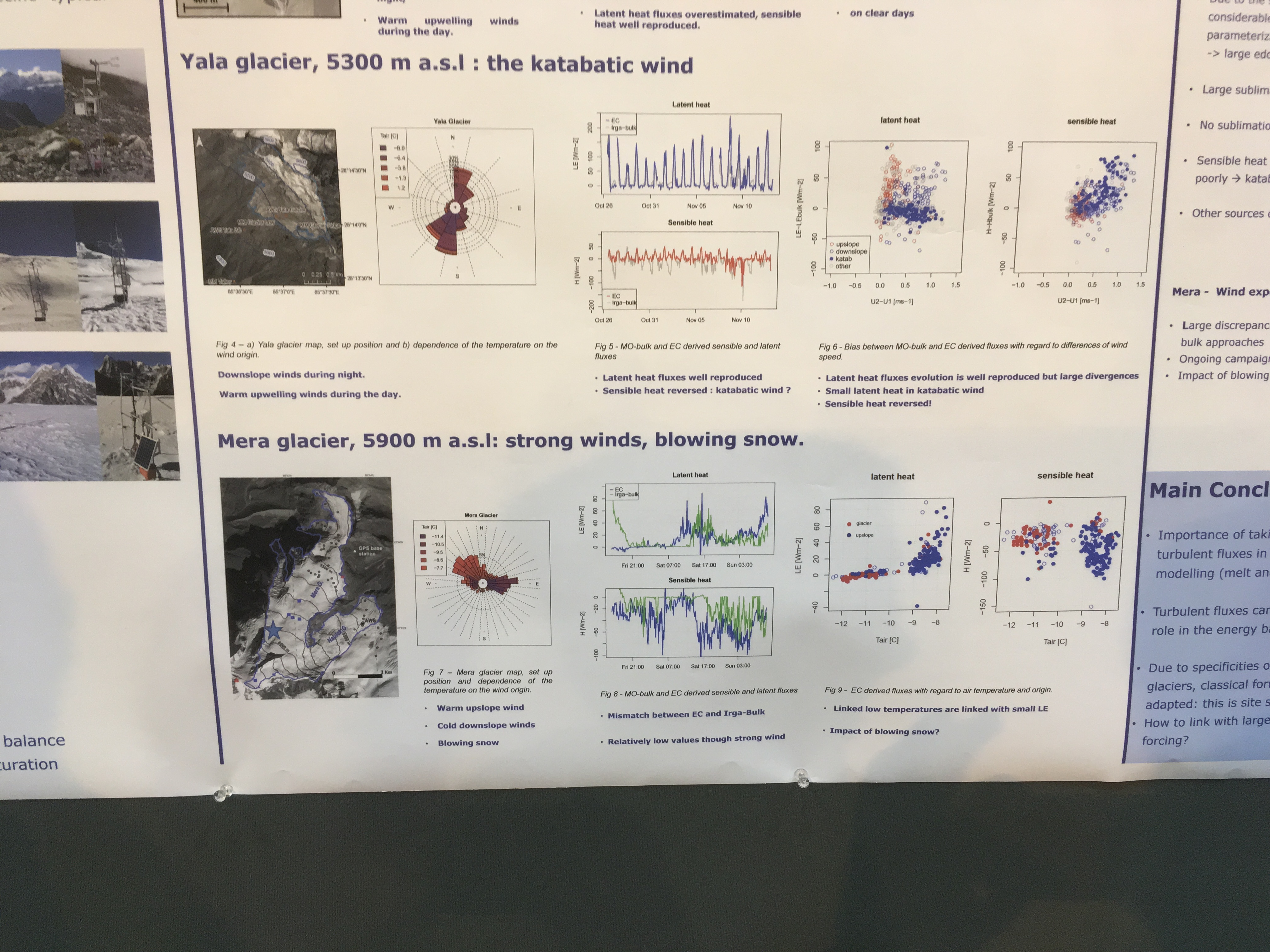
Maxime Litt, Utrecht University installed an eddy-correlation system (Campbell IRGASON) during a period of 15 days over the Lirung glacier in the Langtang Valley in Nepal , during the transition period between the monsoon and the dry season to examine surface energy balance. Results are also reported from Mera Glacier and Yala Glacier. At Lirung Glacier during the day, moderate winds blow up-valley and the atmospheric surface layer is unstable. Latent (sensible) heat fluxes scale between 50 and 150 (50 and 250) Wm^{– 2}during the day, thus drying and cooling the debris and significantly impact SEB. At night, weak down-glacier winds are observed and fluxes remain weak. Yala and Mera Glacier are different environments and illustrate the variations in position on SEB.

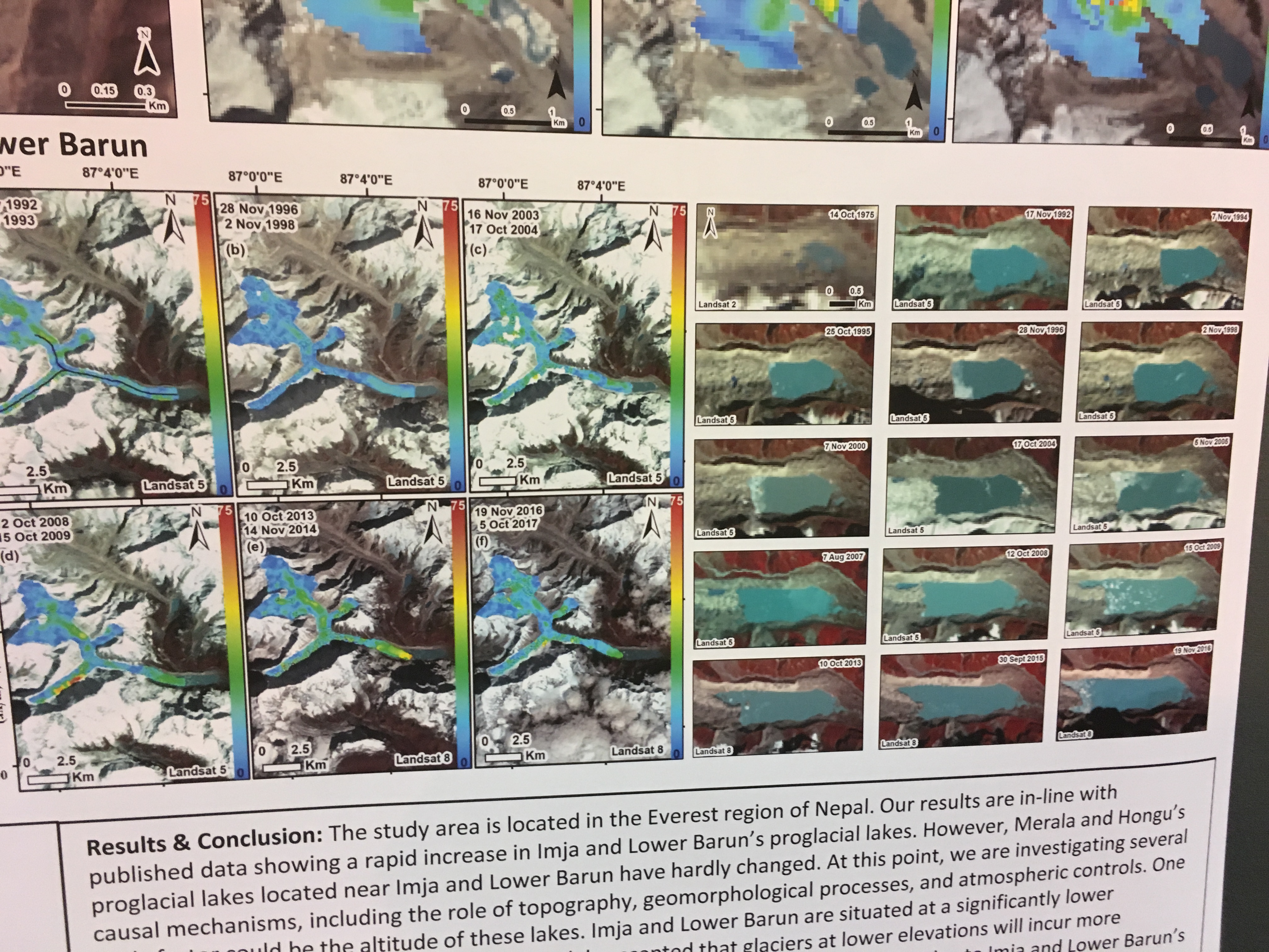
Katherine Strattman, University of Dayton reported on a study of the Imja, Lower Barun, and Thulagi Glaciers in the Nepal Himalaya. The retreat of the glaciers has led to proglacial lakes continuing to dramatically increase in area. They used Landsat, ASTER, and Sentinel satellite imagery to study the conditions of these glaciers. They assessed interannual changes in surface ice velocity from the early 1990s to present. They found both long-term and short-term velocity variations. Satellite imagery indicates the three lakes exhibit three contrasting trends of lake growth: Imja Lake has a strong accelerating growth history since the 1960s, Lower Barun a very slow accelerating growth, and Thulagi a decelerating growth, even as the glaciers of all three lakes have thinned. Above is the velocity of Barun Glacier showing velocity changes and growth of the lake.

Shashank Bhushan, Indian Institute of Technology Dhanbad developed a hazard assessment of moraine dammed glacial lakes in Sikkim Himalayas. They generated high-resolution DEMs using the open-source NASA Ames Stereo Pipeline (ASP) and other open-source tools to calculate surface velocity and patterns of glacier downwasting over time. Geodetic glacier mass balance was obtained for three periods using high-resolution WorldView/GeoEye stereo DEMs, Cartosat-1 stereo DEMs and SRTM. Initial results revealed a region-wide negative annual mass balance of -0.31± m w.eq. for the 2007-2015 period.

Canadian Columbia River Basin Winter 2016-2017: A Late Rally

On August 14, 2017April 28, 2024 By mspeltoIn Glacier Observations, Uncategorized

Guest Post by Ben Pelto, PhD Candidate, UNBC Geography, pelto@unbc.ca

As the summer ticks by and the fall glacier field season approaches, I’ve realized that I never put out a winter 2016-2017 synopsis, so, like the snowfall this year, it’s arrived late.

May 2017, Jesse Milner of the ACMG on the Nordic Glacier in front of the “meteor strike” a newly exposed rock face that spalls ice regularly. Photo by Ben Pelto.

Story of the winter

The winter began with an extremely warm November, featuring temperatures 2-5˚C above normal, with greater than average precipitation generally delivered via Pacific storm cycles. Arctic air masses moving south across BC dominated December, with a complete reversal of temperature to well below average temperatures (Figure 1), and drier conditions. By January 1^st the BC River Forecast Center announced that the Columbia River Basin was at 80-88% of normal snowpack (Figure 2).

Figure 1. Maximum temperature anomaly for December 2016. Note Columbia Basin (SE BC) roughly 3˚C below normal (Pacific Climate Impacts Consortium).

Figure 2. January 1^st snow survey data from the BC River Forecast Center. The Columbia River Basin is comprised of the Upper Columbia, East Kootenay, and West Kootenay Basins, which range from 80-88% of normal.

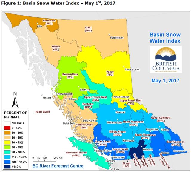
March and April brought cool and moist unstable conditions, leading to a significant increase in snowpack across southern BC, delaying the onset of the melt season by about two weeks. Snowpack measures for the basin were over 100% of normal for the first time of the winter; by May 1^st, the Columbia Basin was at 115% of normal to the north and 135% in the south (Figure 3). By the first week of May, most regions had transitioned into the melt season, though at low to mid-elevations (below 1500 m) much of the snow had already melted.

Figure 3. May 1^st snow survey data from the BC River Forecast Center. The Columbia River Basin is comprised of the Upper Columbia, East Kootenay, and West Kootenay Basins, which ranged from 115 to 137% of normal.

Questions of alpine snowpack conditions

A trend seen over the past few winters is minimal to no snow at lower elevations with significant snow remaining higher, and it’s a pattern expected to continue in an era of rising temperatures leading to both rain on snow, and melt events through the winter. Unfortunately, current measurements, including the network of 70 automatic snow weather stations (ASWS) across the province, are all located at or below 2000 m. This leaves the alpine largely un-sampled. Rising temperatures may well be increasing the balance gradient of winter snow accumulation; that is, there will be a greater rate of change (increase) in snowpack with elevation than previously experienced, though data for this shift is lacking.

Our glacier research program

This information gap of alpine snowpack across BC is being addressed within the context of our glacier mass balance network funded by the Columbia Basin Trust. Each year we have been studying a series of five glaciers across the Basin, which from north to south are the Zillmer Glacier (Valemount), Nordic Glacier (northern boundary of Glacier National Park), Illecillewaet Glacier (Parks Canada, Rodgers Pass, Glacier National Park), Conrad Glacier (Golden, northern boundary of Bugaboo Provincial Park), and the Kokanee Glacier (Nelson, Kokanee Glacier Provincial Park). For more background see previous posts here and here.

Our spring field season consists primarily of snow depth measurements and snow density measurements, used to determine the snow water equivalent (SWE) retained on each glacier at the winter’s end. We also conduct GPS surveys of the glacier height, which we use to account for any surface height change between field visits, and the subsequent airborne laser altimetry surveys (LiDAR)of each glacier and the surrounding area that we’re conducting every spring and fall for the five years of the project.

May 2017, Pulling the ground penetrating radar up the Kokanee Glacier to measure ice thickness. The Kokanee is 20-80 m thick, averaging around 30-40 m. Photo by Rachael Roussin.

Our LiDAR data allows us to calculate snow depth by comparing a fall LiDAR-derived digital elevation model (DEM) to our spring DEM. Off-glacier, the fall DEM represents bare earth, and on glacier, the glacier surface at the end of the melt season. The spring DEM thus captures the fall surface height plus the winter snowpack. The difference in height between the two is taken to be accumulated snow. While our manual snow depth and density surveys of the five study glaciers are incredibly valuable data, our LiDAR surveys cover roughly 10% of the Columbia Basin glacier area, a more than three-fold increase. This expanded footprint allows a better picture of alpine snowpack across the province at elevations largely un-sampled; highly important to downstream concerns such as spring flooding and snow available for summer streamflow.

Fires and Floods

Dramatic swings of weather patterns characterized the 2016-2017 winter, with snowpack well below average in February and early March for the province. By the end of April, snowpack across the Columbia Basin and southern half of the province had rebounded to average or record levels depending upon location with Vancouver and the lower mainland receiving significant snowfall to much fanfare.

The late and cool spring saved the snow season, but also led to flooding across the province, particularly throughout the Okanogan and around Kelowna. As the wildfire season began in earnest, sandbags were still in place in Kelowna to protect properties against flooding from Okanogan Lake, which remained above full pool by 38 cms on July 10^th. Wildfire crews had been tasked with fighting the flooding, and were removing many sandbags as lake levels began to fall before heading off to respond to escalating fires. The flooding began following a rapid warm-up combined with heavy rainfall that led to extreme avalanche risk and activity, with highway closures along the Trans-Canada and Icefields Parkway.

The record snowpack across the southern-most Columbia Basin such as around Nelson, BC, has long since disappeared, with Nelson implementing water restrictions to attempt to cut water usage by 50% in response to the rapidly diminishing snowpack which feed the town’s water supplies.

Forest fires have been raging over the province, burning an area larger than Prince Edward Island, in what is the worst fire season in BC since 1958. Forest fire impact on glaciers is largely unknown, as soot and ash from the fires may raise albedo, but smoke clouds reflect incoming solar radiation. One thing is for certain however, should the fires cloud the skies during our field season, spending 24 hours a day in fire smoke makes for a tough go.

Team members at the foot of a recent avalanche preparing to head up to the Nordic Glacier in the first week of May 2017. Photo by Alex Bevington

Outlook

With our fall field season (August 19-September 21) only a week away, it will be an interesting time to observe how our study glaciers across the Columbia Mountains fared over this roller coaster of a year. After a cold, dry start to the winter, a late rally in March and April delayed the start of the melt season and raised snowpack to well above average across the Columbia Basin. A hot, dry summer led to flooding in May, and now wildfires in June-August, which reversed snowpack levels to below-average at most elevations. Satellite images of the study glaciers show rapidly rising snow lines, as above-average snow packs are reduced to average to below-average across most glaciers, with only the Kokanee Glacier appearing set for a possible positive mass balance year.

How do you get out? Jesse Milner at the bottom of a 5.5 m deep snow pit, which we use for sampling snow density. Nordic Glacier. Photo by Alex Bevington.

The field research is funded by the Columbia Basin Trust, with BC Hydro providing funds for the LiDAR surveys, and addition research support from the Natural Sciences and Engineering Research Council of Canada and the Canada foundation for innovation. The author is a supported by a Pacific Institute for Climate Solutions Fellowship and a scholarship from the University of Northern British Columbia.

Mensu Glacier, Siberia Russia Retreat 1994-2016

On June 27, 2017April 28, 2024 By mspeltoIn climate change glacier retreat, glacier climate change, Glacier Observations, russia glacier retreat

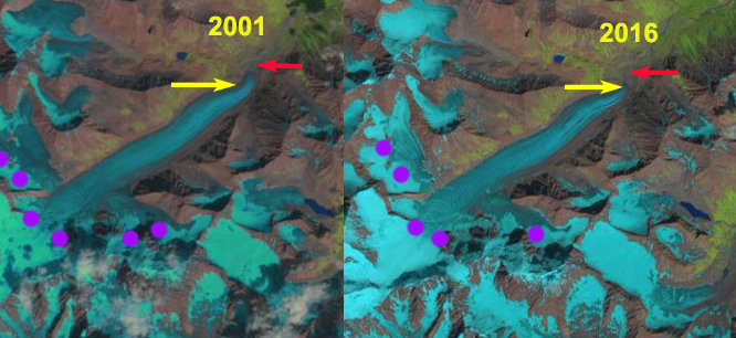
Mensu Glacier, Russia in comparison of 1994 and 2016 Landsat images. Red arrow is the 1994 terminus, yellow arrow 2016 terminus, purple arrow a tributary and purple dots the snowline.

Mensu Glacier (Lednik Mensu) drains northeast from Gora Belukha in the Russian Altai. The glacier drains into the Ob River and then the Arctic Ocean. This glacier has not been the focus of detailed research to date. Khromova et al (2014) report that at the end of the century the glacier degradation in Russian mountain ranges strengthened including glacier area loss of 13% in the Tien Shan, 19% in the Altai and 22.3% in the Polar Urals. The icecap draining west from Gora Belukha was cored to look at longer term climate records (Fujita et al 2004). The core at 4500 m is high enough so that significant melt events affecting the record were rare. Shahgedanova et al (2010) noted that the retreat has largely been driven by summer warming.

In 1994 the glacier terminates at the red arrow at 2150 m. The glacier has an icefall from 3200 m to 2700 m that generates annual ogives, note Google Earth image below. The snowline in the 1994 Landsat image averages 3000 m. There is a tributary joining the main glacier at the purple arrow. A neighboring glacier terminates in a proglacial lake at the orange arrow. By 2001 the glacier has retreated and the snowline is at 3100 m. By 2016 the glacier terminates at 2200 m and has retreated 600 m to the yellow arrow. The tributary at the purple arrow has separated from the main glacier. This illustrates substantial glacier thinning 6 km above the terminus. The glacier at the orange arrow no longer reaches the proglacial lake. In August 2016 below the snowline is at 3100 m in September 2016 the snowline has descended to 2800 m. The lowest 800 m of the glacier has few crevasses, appears stagnant and will be lost to retreat.

Retreat is similar to the nearby Potanin Glacier, Mongolia.

Mensu Glacier, Russia in comparison of 2001 and 2016 Landsat images. Red arrow is the 1994 terminus, yellow arrow 2016 terminus, purple arrow a tributary and purple dots the snowline.

Google Earth image indicating the snowline at the top of the icefall and the ogives beginning at the bottom near the orange arrow.

Terminus of Mensu Glacier in 2013 note lack of crevassing.

Llewellyn Glacier, BC Proglacial Lake Merging From Retreat

On June 5, 2017April 28, 2024 By mspeltoIn Canada glacier retreat, glacier climate change, Glacier Observations

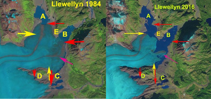
Llewellyn Glacier comparison in 1984 Landsat and 2016 Sentinel images. Red arrows the 1984 terminus locations for proglacial lakes A-D, yellow arrows the 2016 terminus locations for A and B. Point E was the peninsula separating proglacial lakes A and B, which are now joined due to glacier retreat.

The second largest glacier of the Juneau Icefield is the Llewellyn Glacier which is in British Columbia. The Juneau Icefield Research Program has a research camp, C-26 on this glacier and it is the typical exit route from the icefield at the end of the field season. Here we examine changes in the terminus from 1984-2016 as a result of higher snowlines indicative of an expanded ablation zone and negative mass balance.

I first visited the glacier in 1981 and I was also on the icefield in 1984 when the Landsat image was acquired that is used as the start point for comparison. In 1984 the glacier had several termini ending in proglacial lakes A-D. We exited the glacier on the west side of proglacial lake A in 1984 onto a proglacial outwash plain referred to as the ball bearing highway. At Point B the terminus ended in a deeper wider proglacial lake than Lake A. At Point C and D the glacier ended in a series of small lakes. Point E is the peninsula separating proglacial lake A and B in 1984. Proglacial Lake B had a surface water level 10-15 m higher than Lake A in 1984. In 2011 the glacier still reached Point E separating the two lakes, which still had different water levels. In 2013 the gap first opened between the two lakes, and the water level fell in Lake B. In the summer of 2016 and spring of 2017 the gap has persisted and widened to 150 m. From 1984 to 2016 the terminus in Lake A has retreated 1300 m, the terminus at Lake B 2100 m, terminus at Point C 800 m and terminus at Point D 1100 m. The narrow tongue of ice at the pink arrow will not survive long. The crevasse pattern suggests the glacier has another 1.5- 2 km to retreat before lake development will cease.

The snowline during the 1998-2013 period averaged 1900 m too high for an equilibrium balance. In a sequence of images from 2013 illustrates the rise is snowline from 1450 m on June 21, to 1780 m on August 1 and 1810 m on Sept. 2. The persistently higher snowlines since 1990 have led substantial thinning, Melkonian et al. (2013) note thinning of more than 1 m per year at the terminus diminishing to little change above 1500 m from 2000-2009. This will drive continued retreat, supplemented by calving into the still growing proglacial Lake at Point A and B. The retreat of this glacier follows that of other glaciers of the Juneau Icefield including nearby Tulsequah Glacier, noted by Pelto et al (2013) and Pelto (2016) .

[ngg_images source=”recent_images” display_type=”photocrati-nextgen_basic_slideshow” gallery_width=”600″ gallery_height=”400″ cycle_effect=”fade” cycle_interval=”5″ show_thumbnail_link=”1″ thumbnail_link_text=”[Show thumbnails]” order_by=”sortorder” order_direction=”ASC” returns=”included” maximum_entity_count=”4″]

A River Runs 40 km Across the Greenland Ice Sheet

On February 27, 2017May 1, 2024 By mspeltoIn glacier climate change, Glacier Observations, Greenland glacier retreat

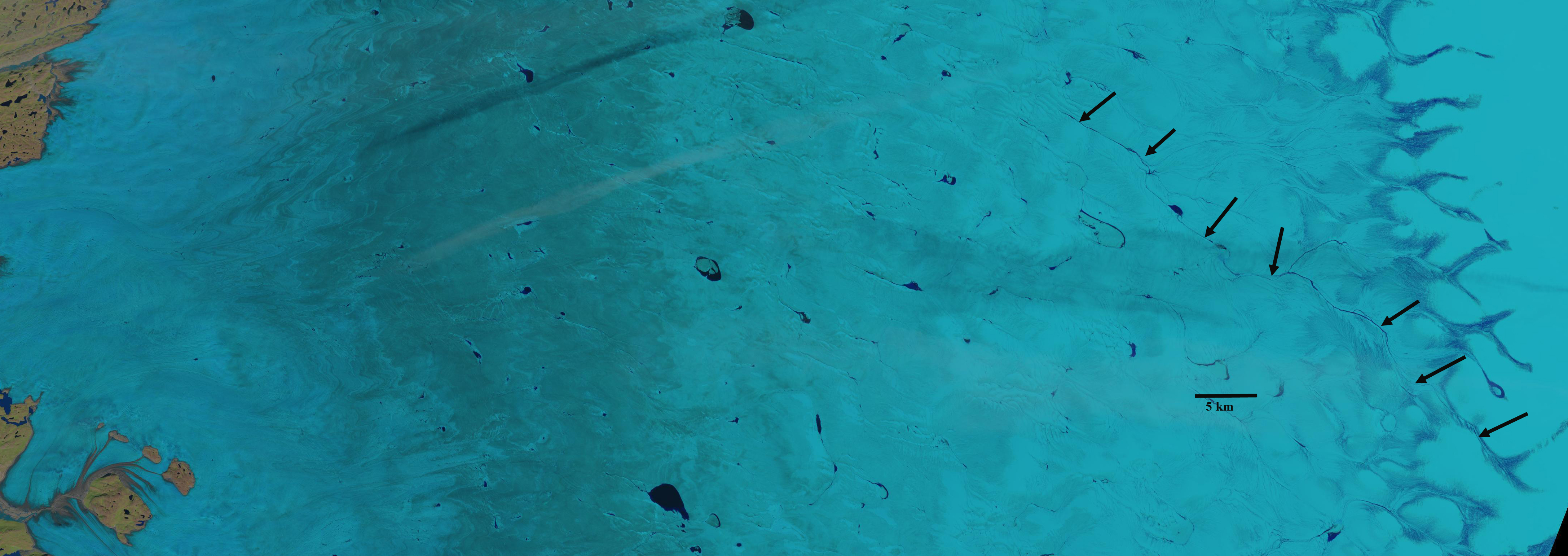
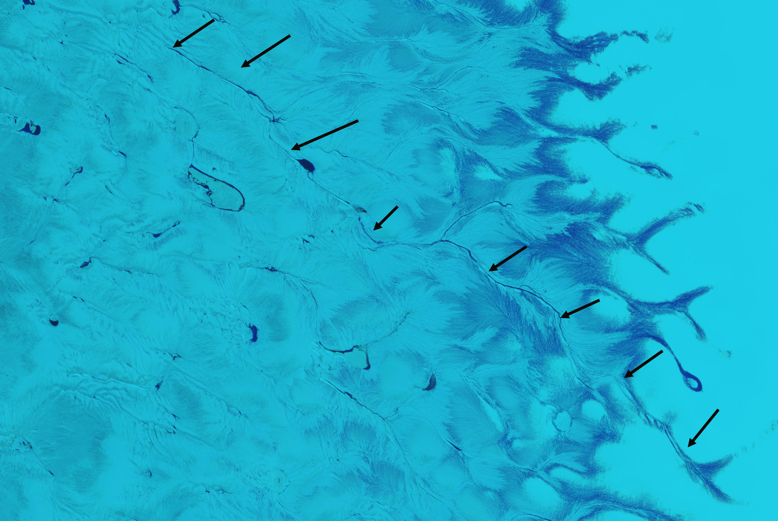
Supraglacial stream, on July 26, 2016 Landsat image, stretching 40 km across the ice sheet from the transient snowline, which marks the boundary between the percolation zone and the wet snow zone, west toward the ice sheet margin, note black arrows.

The Greenland Ice Sheet has experienced a significant increase in surface melt. This is due both to warmer temperatures and enhanced melt due to a reduction in reflectivity-albedo. The expansion in melt area, duration and intensity (NSIDC, 2015) has also generated large volume of meltwater transported via supraglacial streams. Recent work by Tedesco et al (2016) and Kintisch et al (2017) illustrate three key reasons for the albedo change in the melt zone.

1) Upon melting and refreezing, ice crystals lose their branched shape, grow larger and rounder, which reduces the reflectivity of the snow by as much as 10%.

2) Satellite data show that the margins of the ice sheet have darkened by as much as 5% per decade since 2001. Dust trapped over the centuries has become concentrated at the melting edge of the ice sheet.

3) The combination of algae and bacteria with dust generates a sludge—known as cryoconite. This dark material gathers in depressions decreasing albedo. Black and Bloom is a project focused on how dark particles (black) and microbial processes (bloom) darken and accelerate the melting of the Greenland Ice Sheet

Tedesco et al (2016) noted the negative trend in albedo is confined to the regions of the ice sheet that experience summer melting. They also observed no trend during the 1981–1996 period. Their analysis indicates the albedo decrease is due to the combined effects of increased air temperatures, which enhances melt promoting growth in snow grain size and the expansion of bare ice areas, and to increasing concentration of dark impurities on ice surfaces. Kintisch et al (2017) noted the same mechanisms with warmer summers also enhancing microbes and algae growth on the wetter surface of the ice, producing more cryocontie, that reduces albedo absorbing more solar energy. Cryoconite is more spatially limited than the other mechanisms. They also observed that soot and dust that blow in from lower latitudes and darken the ice are also increasing.

The darker surface enhances melt which generates more meltwater largely drained in the melt zone by supraglacial streams. Smith et al (2015) documented the surface drainage in the ablation zone of the southwest GIS. They focused on documenting the distribution of over 500 high order stream channel networks in a 6812 square kilometer region, inland from Kangerlussuaq. All of the stream networks terminated in moulins before the ice sheet edge (NASA, 2015). This indicates that moulins are common, important and sparse.

Poinar et al (2015) observe the longest streams in the 30-50 km range. Here we examine two streams one in detail using Google Earth that is 30 km long and a 40 km long surface stream in 2016 observed in Sentinel 2 and Landsat images. That the surface rivers can travel this distance across the surface before draining via a moulin indicates that the glacier is not structurally like Swiss cheese (Pelto, 2015). The Google Earth detailed view illustrates both the darker surface, the maturity and hydrologic efficiency of the thermally incised meltwater streams.

The stream observed in Google Earth in its mid-reach has an average of 15 m in width. The slope of the ice sheet is 1/120 in this region, with the river beginning at 1320 m and ending at 1070 m. Gleason et al (2016) examined numerous supraglacial streams and noted that supraglacial streams with a width of 15-20 m and slopes of 1/100 to 1/200 had a depth of 1.5-2.0 m and velocity of ~0.5 m/sec. This suggests the stream here has a discharge of 7-10 cubic meters per second. The darkness of the ice surface indicating a low albedo is also apparent. The ice is not nearly as dark when standing directly on it as it is in the macro-scale.

[ngg_images source=”galleries” container_ids=”52″ display_type=”photocrati-nextgen_basic_imagebrowser” ajax_pagination=”1″ template=”/nas/wp/www/sites/blogsorg/wp-content/plugins/nextgen-gallery/products/photocrati_nextgen/modules/ngglegacy/view/imagebrowser-caption.php” order_by=”sortorder” order_direction=”ASC” returns=”included” maximum_entity_count=”500″]

The second stream is seen in a Sentinel image from July 15 and a Landsat image from July 26. The black arrow indicate the stream that is 40 km long. The stream extends from 110 km from the edge of the ice sheet to within 75 km. The stream begins near the transient snowline at 1650 m and ends near 1400 m, creating a slushy valley above the local percolation zone. The stream in early July flows through the wet snow zone. By the end of the July the lower section of the stream becomes a bare ice region, the upper remains in the wet snow zone.

Supraglacial stream in mid-July Sentinel images stretching 40 km across the ice sheet from the transient snowline west toward the ice sheet margin.

State of Alpine Glaciers in 2016-Negative for 37th Consecutive Year

On February 17, 2017May 1, 2024 By mspeltoIn climate change glacier retreat, glacier climate change, Glacier Observations

Figure 1. Global Alpine glacier annual mass balance record of reference glaciers submitted to the World Glacier Monitoring Service.

Each year I write the section of the BAMS State of the Climate on Alpine Glaciers. What follows is the initial draft of that with a couple of added images and an added paragraph.

The World Glacier Monitoring Service (WGMS) record of mass balance and terminus behavior (WGMS, 2015) provides a global index for alpine glacier behavior. Globally in 2015 mass balance was -1177 mm for the 40 long term reference glaciers and -1130 mm for all 133 monitored glaciers. Preliminary data reported to the WGMS from Austria, Canada, Chile, China, France, Italy, Kazakhstan, Kyrgyzstan, Norway, Russia, Switzerland and United States indicate that 2016 will be the 37^th consecutive year of without positive annual balances with a mean loss of -852 mm for reporting reference glaciers.

Alpine glacier mass balance is the most accurate indicator of glacier response to climate and along with the worldwide retreat of alpine glaciers is one of the clearest signals of ongoing climate change (Zemp et al., 2015). The ongoing global glacier retreat is currently affecting human society by raising sea-level rise, changing seasonal stream runoff, and increasing geohazards (Bliss et al, 2014; Marzeion et al, 2014). Glacier mass balance is the difference between accumulation and ablation. The retreat is a reflection of strongly negative mass balances over the last 30 years (Zemp et al., 2015). Glaciological and geodetic observations, 5200 since 1850, show that the rates of early 21st-century mass loss are without precedent on a global scale, at least for the time period observed and probably also for recorded history (Zemp et al, 2015). Marzeion et al (2014) indicate that most of the recent mass loss, 1991-2010 is due to anthropogenic forcing.

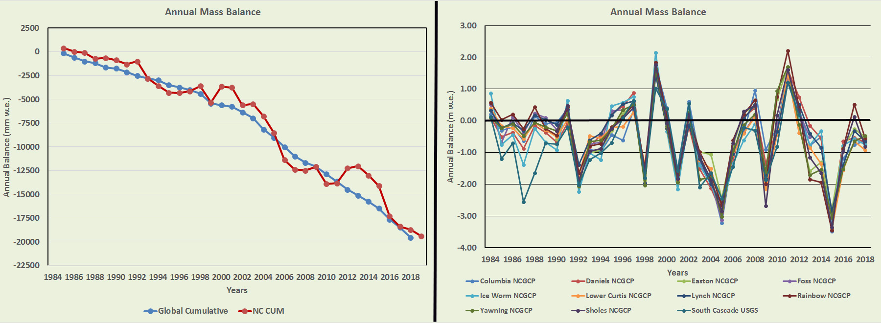
The cumulative mass balance loss from 1980-2015 is -18.8 m water equivalent (w.e.), the equivalent of cutting a 21 m thick slice off the top of the average glacier (Figure 2). The trend is remarkably consistent from region to region (WGMS, 2015). WGMS mass balance based on 40 reference glaciers with a minimum of 30 years of record is not appreciably different from that of all glaciers at -18.3 m w.e. The decadal mean annual mass balance was -228 mm in the 1980’s, -443 mm in the 1990’s, –676 mm for 2000’s and – 876 mm for 2010-2016. The declining mass balance trend during a period of retreat indicates alpine glaciers are not approaching equilibrium and retreat will continue to be the dominant terminus response. The recent rapid retreat and prolonged negative balances has led to some glaciers disappearing and others fragmenting (Figure 2)(Pelto, 2010; Lynch et al, 2016).

Below is a sequence of images from measuring mass balance in 2016 in Western North America from Washington, Alaska and British Columbia. From tents to huts, snowpits to probing, crevasses to GPR teams around the world are assessing glacier mass balance in all conditions.

[ngg_images source=”galleries” container_ids=”7″ display_type=”photocrati-nextgen_basic_imagebrowser” ajax_pagination=”1″ template=”/nas/wp/www/sites/blogsorg/wp-content/plugins/nextgen-gallery/products/photocrati_nextgen/modules/ngglegacy/view/imagebrowser-caption.php” order_by=”sortorder” order_direction=”ASC” returns=”included” maximum_entity_count=”500″]

Much of Europe experienced record or near record warmth in 2016, thus contributing to the negative mass balance of glaciers on this continent. In the European Alps, annual mass balance has been reported for 12 glaciers from Austria, France, Italy and Switzerland. All had negative annual balances with a mean of -1050 mm w.e. This continues the pattern of substantial negative balances in the Alps continues to lead to terminus retreat. In 2015, in Switzerland 99 glaciers were observed, 92 retreated, 3 were stable and 4 advanced. In 2015, Austria observed 93 glaciers; 89 retreated, 2 were stable and 2 advanced, the average retreat rate was 22 m.

In Norway, terminus fluctuation data from 28 glaciers with ongoing assessment, indicates that from 2011-15 26 retreated, 1 advanced and 1 was stable. The average terminus change was -12.5 m (Kjøllmoen, 2016). Mass balance surveys with completed results are available for seven glaciers; six of the seven had negative mass balances with an average loss of -380 mm w.e.

In western North America data has been submitted from 14 glaciers in Alaska and Washington in the United States, and British Columbia in Canada. All 14 glaciers reported negative mass balances with a mean loss of -1075 mm w.e. The winter of and spring of 2016 were exceptionally warm across the region, while ablation conditions were close to average.

In the high mountains of central Asia five glaciers reported data from Kazakhstan, Kyrgyzstan and Russia. Four of five were negative with a mean of -360 mm w.e. Maurer et al (2016) noted that mean mass balance in the eastern was significantly negative for all types of glaciers in the Eastern Himalaya from 1974-2006.

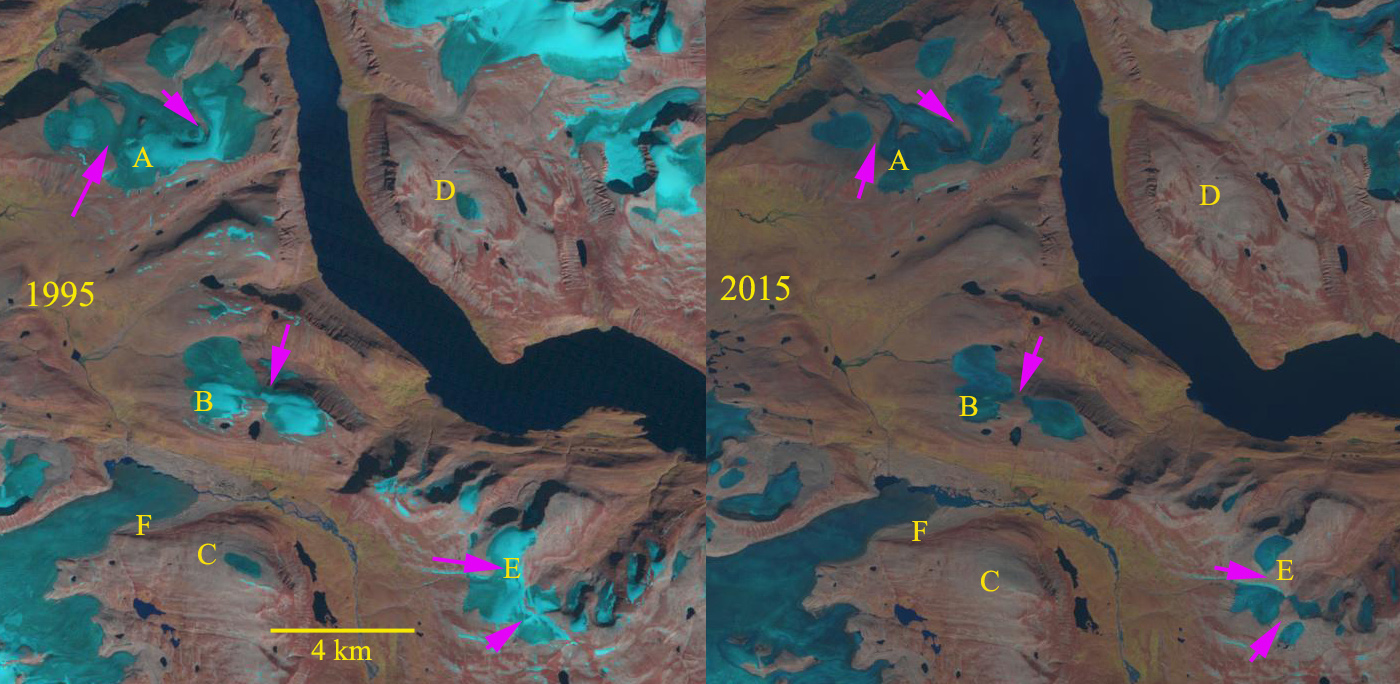
Figure 2. Landsat images from 1995 and 2015 of glaciers in the Clephane Bay Region, Baffin island. The pink arrows indicate locations of fragmentation. Glaciers at Point C and D have disappeared.

Recent Climate Change Impacts on Mountain Glaciers-Mauri Pelto

On February 4, 2017May 1, 2024 By mspeltoIn Glacier Observations

Book Description:

Recent Climate Change Impacts on Mountain Glaciers-Mauri Pelto

Glaciers are considered a key and an iconic indicator of climate change. The World Glacier Monitoring Service has noted that global alpine balance has been negative for 35 consecutive years. This highlights the dire future that alpine glaciers face.

The goal of this volume is to tell the story, glacier by glacier, of response to climate change from 1984-2015. Of the 165 glaciers examined in 10 different alpine regions, 162 have retreated significantly. It is evident that the changes are significant, not happening at a “glacial” pace, and are profoundly affecting alpine regions. There is a consistent result that reverberates from mountain range to mountain range, which emphasizes that although regional glacier and climate feedbacks differ, global changes are driving the response. This book considers ten different glaciated regions around the individual glaciers, and offers a different tune to the same chorus of glacier volume loss in the face of climate change. Below are some sample image pairs all Landsat images from the book. The red arrow indicates the earlier terminus, yellow arrow later terminus position and purple arrows upglacier thinning.

I continue to post two blogs a week on glaciers at https://glacierchange.blog/

Continue reading “Recent Climate Change Impacts on Mountain Glaciers-Mauri Pelto” →

Recent Climate Change Impacts on Mountain Glaciers – Volume

On January 12, 2017May 1, 2024 By mspeltoIn glacier climate change, Glacier Observations

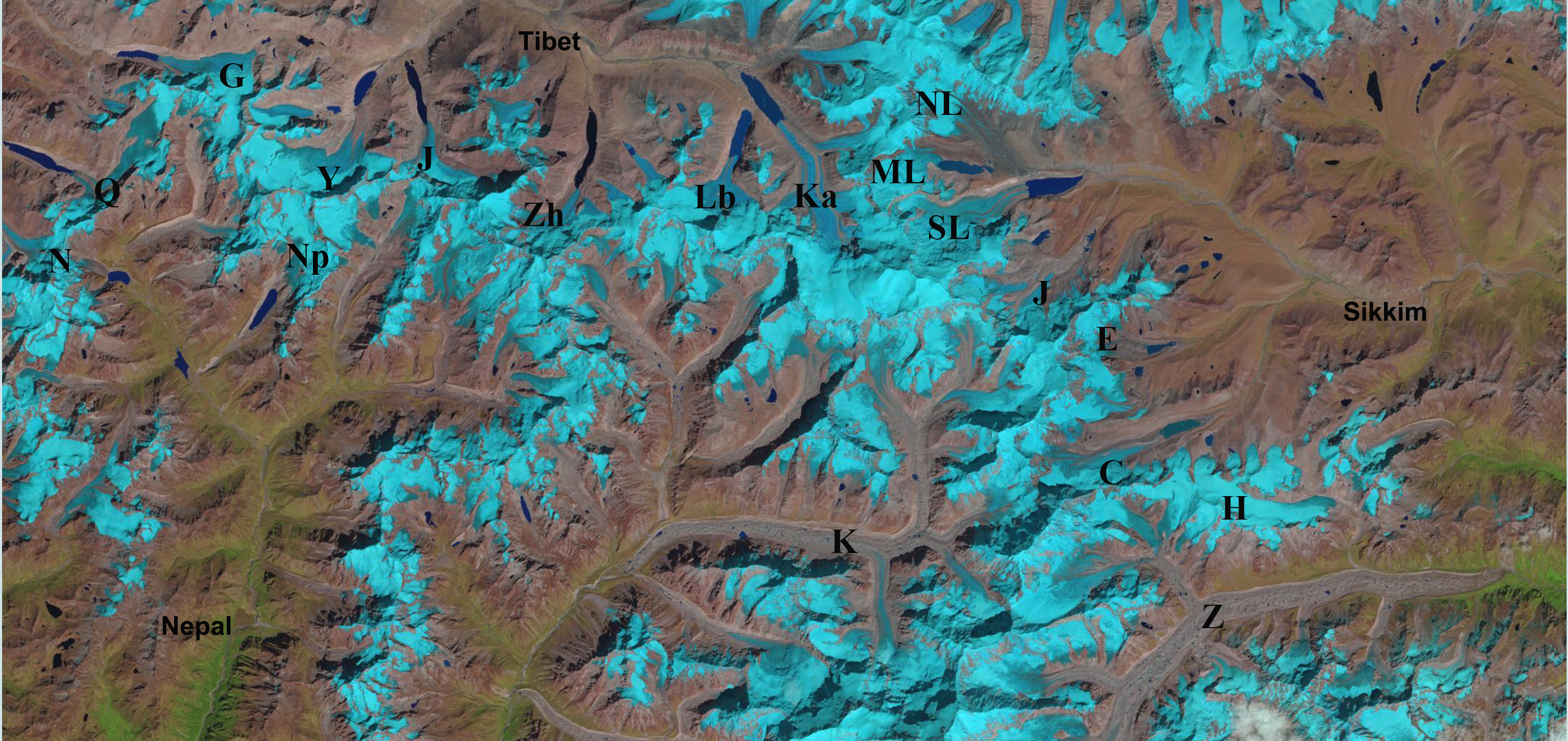
Landsat Image of glaciers examined in the Himalaya Range: Chapter 10 that straddles a portion of Sikkim, Nepal and Tibet, China. Notice the number that end in expanding proglacial lakes.

This January a book I authored has been published by Wiley. The goal of this volume is to tell the story, glacier by glacier, of response to climate change from 1984-2015. Of the 165 glaciers examined in 10 different alpine regions, 162 have retreated significantly. It is evident that the changes are significant, not happening at a “glacial” pace, and are profoundly affecting alpine regions. There is a consistent result that reverberates from mountain range to mountain range, which emphasizes that although regional glacier and climate feedbacks differ, global changes are driving the response. This book considers ten different glaciated regions around the individual glaciers, and offers a different tune to the same chorus of glacier volume loss in the face of climate change. There are 107 side by side Landsat image comparisons illustrating glacier response. Several examples are below: in each image red arrows indicate terminus positions from the 1985-1990 period and yellow arrows terminus positions for the 2013-2015 period, and purple arrows upglacier thinning.

[ngg_images source=”galleries” container_ids=”17″ display_type=”photocrati-nextgen_basic_imagebrowser” ajax_pagination=”1″ template=”/nas/wp/www/sites/blogsorg/wp-content/plugins/nextgen-gallery/products/photocrati_nextgen/modules/ngglegacy/view/imagebrowser-caption.php” order_by=”sortorder” order_direction=”ASC” returns=”included” maximum_entity_count=”500″]

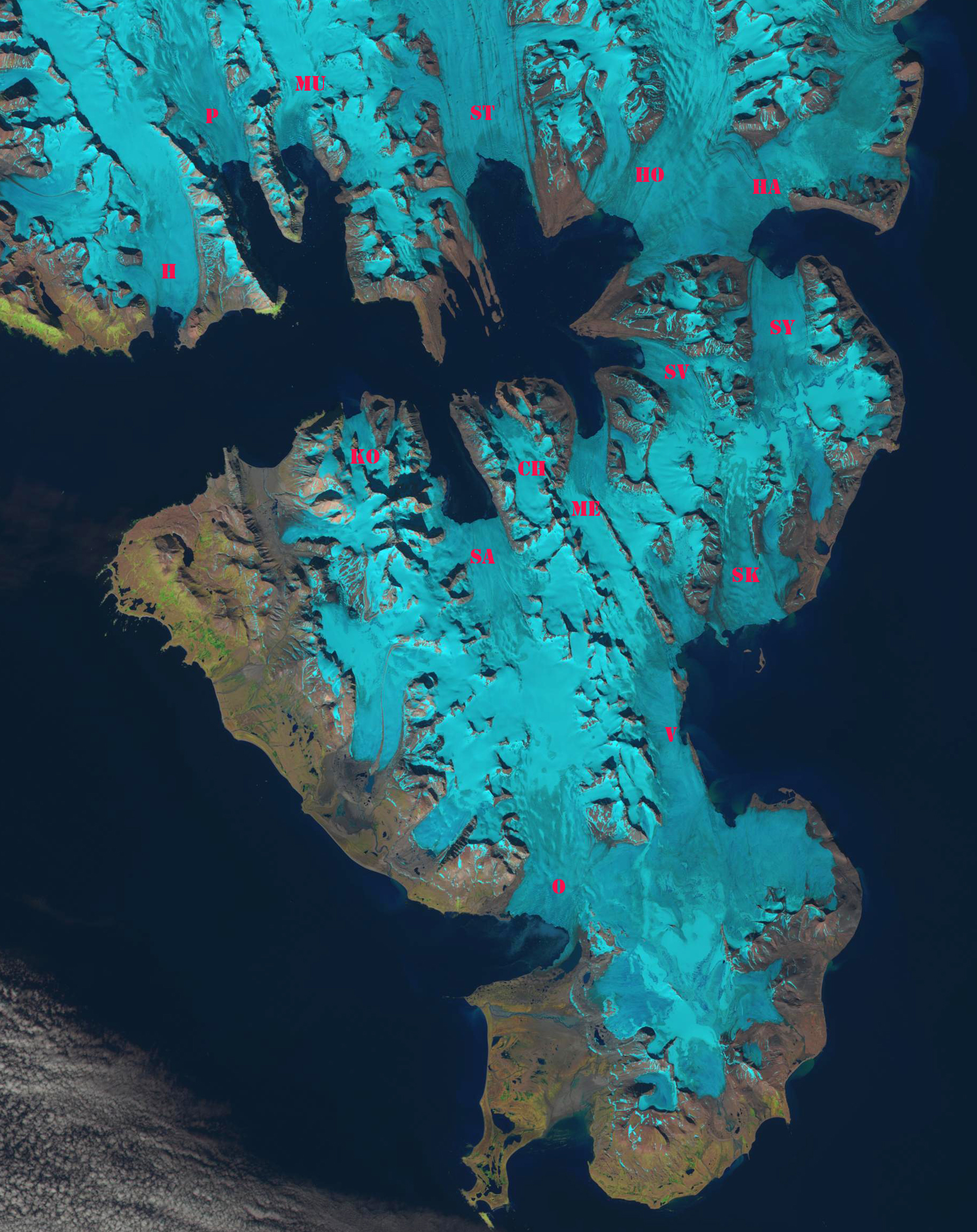
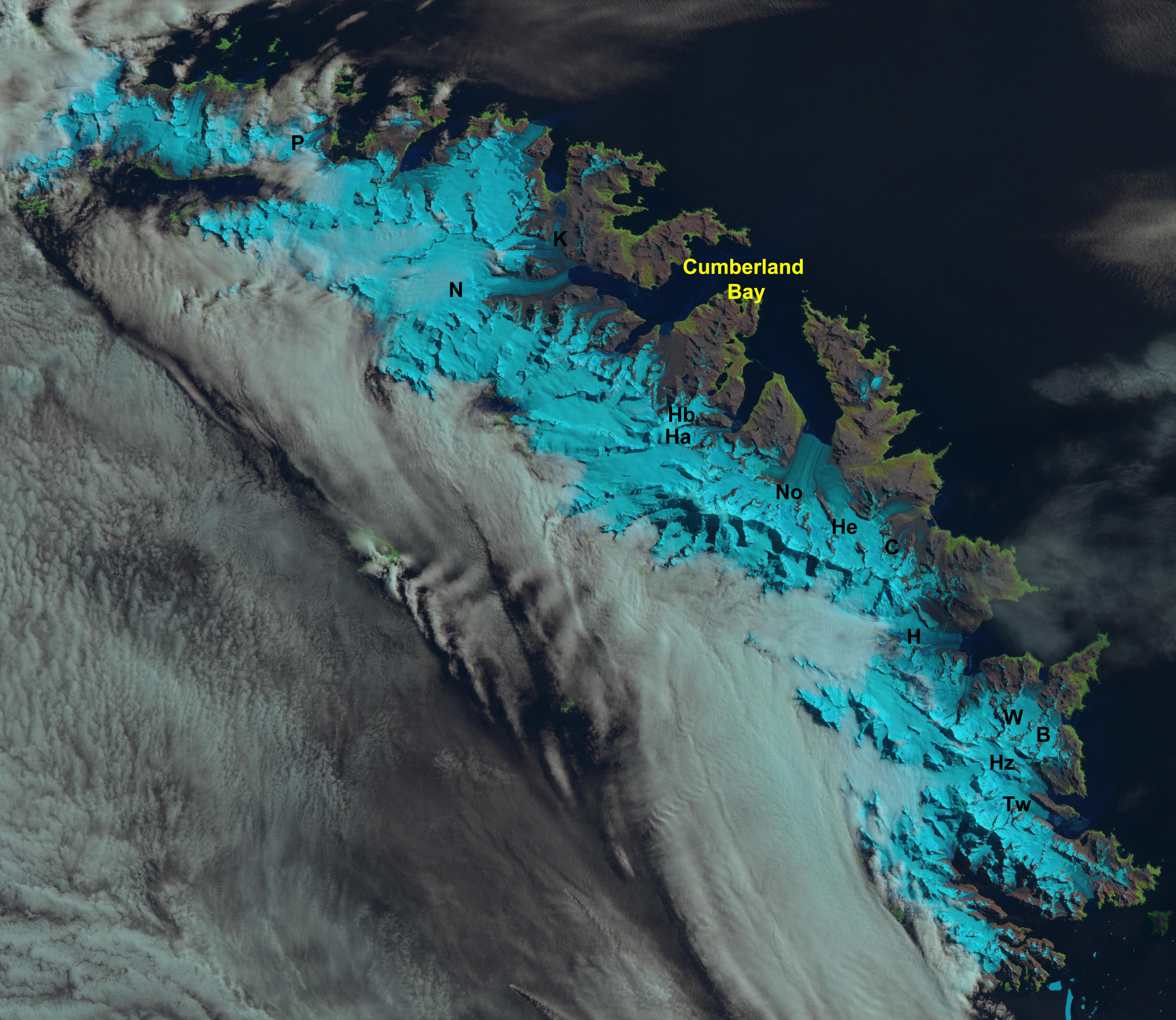
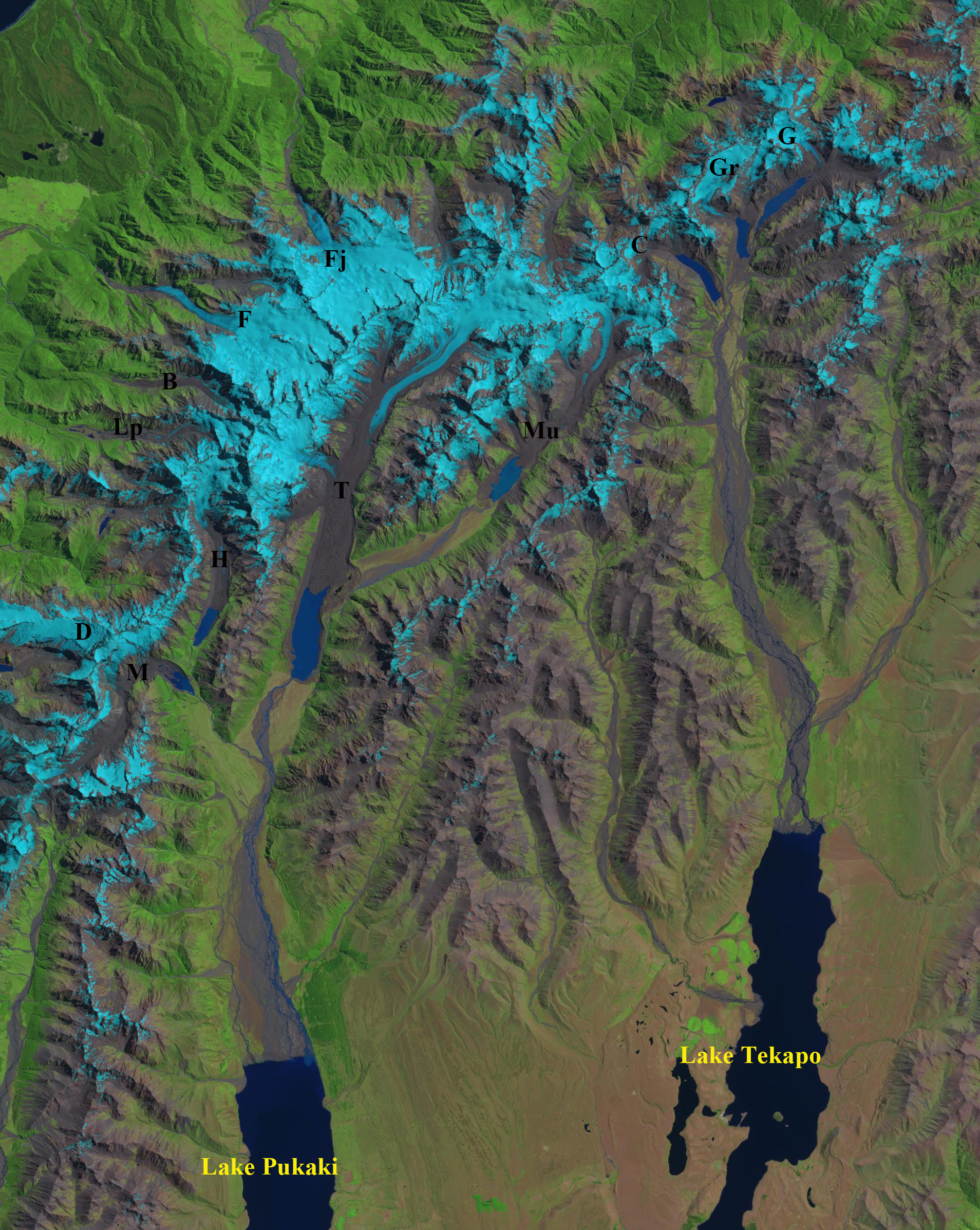
There are chapters on: Alaska, Patagonia, Svalbard, South Georgia, New Zealand, Alps, British Columbia, Washington, Himalaya, and Novaya Zemlya. If you are a frequent reader of this blog you will recognize many of the locations. This updates each glacier to the same time frame. The book features 100 side by side Landsat image pairs illustrated using the same methods to illustrate change of each glacier. The combined efforts of the USGS and NASA in obtaining and making available these images is critical to examining glacier response to climate change. The World Glacier Monitoring Service inventory of field observations of terminus and mass balance on alpine glaciers is the another vital resource. The key indicators that glaciers have been and are being significantly impacted by climate change are the global mass balance losses for 35 consecutive years documented by the WGMS. The unprecendented global retreat that is increasing even after significant retreat has occurred in the last few decades (Zemp et al, 2015). Last, the decline in area covered by glaciers in every alpine region of the world that is documented by mapping inventories such as the Randolph Glacier inventory and GLIMS ( Kargel et al 2014)

Landsat Image of glaciers examined in the Svalbard: Hornsund Fjord Region: Chapter 6.

Landsat Image of glaciers examined in the South Georgia Island: Chapter 5.

Landsat Image of Mount Baker glaciers examined in the North Cascades, Washington: Chapter 8.

Landsat Image of glaciers examined in the Southern Alps of New Zealand S: Chapter 11.

Gangotri Glacier Expanded Melt Season & Melt Area in 2016

On January 4, 2017May 1, 2024 By mspeltoIn glacier climate change, Glacier Observations, Himalaya glacier retreat

[ngg_images source=”galleries” container_ids=”22″ display_type=”photocrati-nextgen_basic_imagebrowser” ajax_pagination=”1″ template=”/nas/wp/www/sites/blogsorg/wp-content/plugins/nextgen-gallery/products/photocrati_nextgen/modules/ngglegacy/view/imagebrowser-caption.php” order_by=”sortorder” order_direction=”ASC” returns=”included” maximum_entity_count=”500″]

Purple dots indicate the transient snowline on Gangotri Glacier in the fall and early winter of 2016. Red arrow indicates the terminus of the glacier.

The Gangotri Glacier is the largest glacier in the Bhagirathi River watershed, situated in the Uttarkashi District, India. It is one of the larger glaciers in the Himalaya, and like all of the nearby Himalayan glaciers is retreating significantly. Gangotri Glacier provides hydropower as its meltwater passes through three hydropower plants generating 1430 MW, including the 1000 MW Tehri Dam and reservoir and Maneri Bhali I and II, see map below. From 1968-2006 the glacier retreated 800 meters, close to 20 meters per year (Bhambri et al, 2012). The glacier continues to thin and tributary inflow decline, while terminus retreat is slowe due to the thick debris cover that heavily insulates the ice. Bhambri et al (2011) inventoried glaciers in the upper Bhagirathi basin and found they lost 9 square kilometers in area, 3.3% to the total, from 1968 to 2006. They further noted that recession rates have increased since 1990 and that the number of glaciers increased from 82 in 1968 to 88 in 2006 due to fragmentation of glaciers. From 1968 to 2006, the debris-covered glacier area increased by ~12% in the upper Bhagirathi basin. Bhattachaya et al (2016) expanded on this work noting that the velocity of Gangotri Glacier declined during 2006-2014 by 6.7% from 1993-2006, this suggests reduced accumulation being funneled downglacier. They also noted an increase in the rate of debris-covered area expansion on the main trunk of Gangotri Glacier from 2006-2015, which is indicative of an expanding ablation zone. Bhattachaya et al (2016) report a retreat rate of 9 m/year 2006-2015, which is less than before, but the down-wasting in the same period 2006-2015 was higher than during 1968-2006. The study reinforced that glacier retreat is a delayed response to climate change, whereas glacier mass balance is a more direct and immediate response. This underlines the importance of mass balance studies for assessing climate change impact on glaciers,that the World Glacier Monitoring Service has emphasized. Gangotri Glacier is a summer accumulation glacier with the peak ablation period low on the glacier coinciding with peak snowfall high on the glacier during the summer monsoon. In the post monsoon period of October and November precipitation is low and melt rates decline, Haritashya et al (2006) note a sharp decline in discharge and suspended sediment load beginning in October. . Kundu et al (2015) from Sept. 2012 to January 2013 noted that the snowline elevation varied little, with the highest elevation being 5174 m and the lowest 5080 m.

The increase in temperature has led to a tendency for snowlines to rise in the post monsoon period and remain high into the winter season on many Himalayan glaciers. In 2016 this has been the case. On October 9, 2016 a Sentinel image indicates the snowline is at 4850 m on the main trunk and on the tributary Ghanohim Glacier the snowline, while it is 4750 m on the tributaryKirti Glacier. A Landsat image from October 13th indicates the snowline on Kirti has risen to 4800 m, and remains at 4850 on the main trunk and Ghanohim Glacier. By November 30th a Landsat image indicates the snowline has risen to 5400 m on the main trunk and Ghanohim, the snowline is at 5800-5900 m on the glaciers in the Swachhand tributary valley, at 5600 m on Maiandi Glacier and 5700 m on the last tributary entering from the north. Note the impact of radiational shading is apparent on the main trunk with the snowline descending down the middle of the main trunk from 5400 m to 5100 m and on Kirti Glacier which is too dark to confidently discern the snowline. Temperatures are typically cool in December, but sunshine is common. A Sentinel image from December 8th and Landsat from Dec. 9th indicate that the snowline remains approximately the same as on Nov. 30th. The accumulation area ratio is the percentage of a glacier in the accumulation zone and is typically above 50%. On Gangotri Glacier in December 2016 the accumulation area ratio is only 20%, indicating a large mass balance deficit. High winter snowlines on Chutenjima Glacier, Tibet, from October, 2015 to February 2016. This tendency is also noted at Nup La-West Rongbuk Glacier, on the Nepal-China border, West Hongu Glacier, Nepal and Lhonak Glacier, Sikkim.

Gangotri Glacier and its key tributaries, with the red line being the outline of the glacier from GLIMS.

Hydropower in the Bhagirathi River watershed

Norrearm Fjord Glacier Retreat, Greenland

On December 9, 2016May 1, 2024 By mspeltoIn glacier climate change, Glacier Observations, Greenland glacier retreat

Apostelens Glacier in Norrearm Fjord Landsat comparison from 1999 to 2016. Red arrows are the 1999 terminus location, yellow arrows the 2016 terminus location and purple arrows indicate an expanding bedrock ridge.

“Apostelens” Glacier drains east from a peak of the same name into an arm of Norrearm Fjord, which in turn is part of Lindenow Fjord in southern Greenland. The glacier is a short distance north of Kangersuneq Qingordleq, where recent retreat has led to glacier separation. The glacier is soon to lose its tidewater connection as has occurred at Tasermiut Fjord to the west. This will result in a decline in iceberg production as well.

Here we examine Landsat imagery from 1999-2016 to identify glacier change. In 1999 the Apostelens arm of Norrearm Fjord is largely filled by the glacier which extends to within 2.5 km of Norrearm Fjord, red arrow. The tongue contains numerous ogives formed each year due to seasonal velocity changes through an icefall. This is evident in the Google Earth image from 2004, where 24 ogives are evident on the low slope glacier tongue, in 1999 the number is over 30. By 2013 the glacier has retreated nearly 2 km from the 1999 terminus position, red arrow. In 2012 Google Earth imagery indicates increased crevassing near the front and the loss of most ogives. New ogive formation is also hard to distinguish. By 2016 the glacier has retreated 2.6 km and is nearing the headward limit of the fjord arm. The collapse of the fjord tongue and its associated ogives indicates the loss of 30 years worth of volume flux that emerged from the icefall that generated the ogives.

Greenland tidewater outlet glaciers in this region have experienced substantial retreat since 1990, Weidick et al (2012) and Howat and Eddy (2011). Murray et al (2015) examined 199 tidewater glaciers in Greenland and noted significant retreat of 188 of them. Apostelens Glacier was not one of these, and soon will not be a tidewater glacier to be included in the list.

Apostelens Glacier in Norrearm Fjord Google Earth comparison from 2004 and 2012. Red arrows are the 2004 terminus location, and yellow arrows the 2012 terminus location. Note ogives in 2004 and loss of them in 2012.