Glaciar Olvidado, Chile Retreat Lake Expansion 1985-2017

Glaciar Olvidado (O) retreat illustrated in 1985 and 2017 Landsat images.  Red arrow is 1985 terminus location, yellow arrow is 2017 terminus location and purple dots are the snowline.  This illustrates an 1800 m retreat. 

Glaciar Olvidado (G) is a glacier in the southeast portion of the Southern Patagonia Icefield (SPI), adjacent to Grey Glacier (G).  The glacier terminates in a proglacial lake. Rivera and Casassa (2004) report the glacier terminating in a newly formed lake in 1986 and retreating slowly from 1986 to 2000.  Here we examine changes in the glacier from 1985 to 2017 using Landsat imagery.

In 1985 the glacier terminates in small newly formed proglacial lake that is just 200 m long.  The snowline in 1985 is at 1050 m. In 2000 the lake has expanded to a length of 900 m.  The snowline in 2000 is at 950 m.  By 2016 the proglacial lake has expanded to  a length of 2 km.  The snowline in 2016 is at 1100 m.  In 2017 the glacier has retreated 1800 m since 1986.  The snowline is at the base of the steep slopes at 1150 m.  The high snowline leaves less than 30% of the glacier in the accumulation zone.  The high snowlines indicate a limited accumulation zone, which generates a negative mass balance and drives retreat.  The glacier continues to calve into this terminus lake adding to the negative mass balance and consequent retreat.  This glacier adds to the growth of proglacial lakes seen in the Northern Patagonia Icefield  (Glasser et al 2016) and SPI (Iribarren et al 2014).  Olvidado Glacier retreat in terms of distance is similar to the adjacent Grey Glacier, but does represent 20% of its total length.  The retreat is much less than the HPS-12 glacier on the west side of the SPI. 

Glaciar Olvidado retreat illustrated in 2000 and 2016 Landsat images.  Red arrow is 1985 terminus location, yellow arrow is 2017 terminus location and purple dots are the snowline. 

Olvidado Glacier in 2016 Google Earth image. 


Safuna & Arhuey Glacier, Peru Retreat from Lakes

Safuna Glacier (S) and Arhuey Glacier (A) in 1992 and 2017 Landsat images indicating glacier retreat from the 1992 terminus red arrow to the 2017 terminus position yellow arrow.  Snowline indicated by purple dots.

Safuna Glacier (S) is at the northern end of the Cordillera Blanca Range, Peru flowing north from Nevados Pucajirca.  Arhuey Glacier (A) is adjacent to Safuna and flows west formerly terminating in Arhuey Lagunacocha impounded by a moraine. Safuna Glacier in 1992 terminated in Laguna Safuna Alta, which is impounded by a moraine dam and has a history of water level fluctuations.   Reynolds Geosciences (2003) provides a detailed look at the lake, moraine and associated engineering.  The moraine appeared unstable in the 1960’s prompting excavation of  a tunnel through the moraine in 1970, which ended up below the lake water level after the lake surface elevation dropped 25 m in late 1970.  In 1978 a second tunnel was constructed, that to date remains above the lake waterline and has not been used.  The Peruvian Government was early in their proactive engineering to address glacier lake outburst flood hazards (Carey, 2008). In 2002, a rockslide created a wave of at least 80 meters in height (Reynolds Geosciences , 2003), overtopping the moraine and damaging both tunnels but not damaging the moraine.  This landslide also filled in the lake reducing depth significantly. Here we examine changes  from 1992 to 2017 using Landsat imagery from July of Safuna Glacier (S) and Arhuey Glacier (A). Though glacier outburst floods have capture more attention it is the overall reduction in glacier water runoff that has more impact on local communities (GlacierHub-Angle, 2017).

In 1992 the glacier terminated in the 800 m long Laguna Safuan Alta, red arrow .  The lower glacier featured a long narrow valley tongue extending into the lake.  By 1995 retreat had led to further lake expansion, with the glacier still reaching the lake across a narrower front.  In 1996 as was the case in 1992 and 1995 the snowline on the glacier is above the main icefall area where the valley tongue descends from the accumulation zone, purple dots at an elevation of 4950 m. By 2015 the glacier had receded from the shore of the lake and the terminus is covered in debris from the 2002 landslide.  In 2015 and 2016 the snowline is higher than in the 1990  at 5100 m.  In 2017 the glacier terminates 200 m from the lake shore and 500 m from the 1992 terminus location.  The lake is now 1100 m long. The glacier no longer can easily release ice avalanches into the lake

The retreat of this glacier mirrors that of Arhuey Glacier (A), which terminated in the newly forming Arhuey Lagunacocha. By 1995 and 1996 the terminus tongue is more distinct and the lake is 400-500 m long.  By 2015 and 2016 the glacier has retreated to the far end of the lake basin, though still in contact with the lake  By 2017 the lake is 1150 m long, indicating a 700 m retreat since 1992.  The upper portion of the glacier remains incredibly crevassed indicate vigorous accumulation and motion.  The glacier has a relatively small ablation zone with the loss of the flatter terminus reach, and should have a reduced rate of retreat.  The glacier now has a reduced but still significant ability to release ice avalanches into the lake.  The glacier fits into the  Cordillera Blanca regional pattern which has experienced a 22% glacier loss from 1970-2003 (Racoviteanu et al, 2008).

Emmer et al (2016) note that the number of GLOF’s were greater from moraine dammed lakes in the region early in the retreat phase in the 1940’s and 1050’s.  This suggest the moraines are becoming more stable with time since formation and glacier retreat.  The broader impact of climate change is examined by the GlacierHub (Marconi, 2016). 


Safuna Glacier, Laguna Safuna Alta and Laguna Safuna Baja (SB), blue arrow recent 2002 landslide scar and yellow arrow 2017 terminus.


Arhuey Glacier and Arhuey Lagunacocha. Black arrows indicate heavy crevassing, blue arrow recent landslide scars and yellow arrow 2017 terminus.

Safuna Glacier (S) and Arhuey Glacier in 1995 and 2015 Landsat images indicating glacier retreat from the 1992 terminus red arrow to the 2017 terminus position yellow arrow.  Snowline indicated by purple dots.

Safuna Glacier (S) and Arhuey Glacier in 1996 and 2016 Landsat images indicating glacier retreat from the 1992 terminus red arrow to the 2017 terminus position yellow arrow.  Snowline indicated by purple dots.  

Tajuco Glacier Lake, China Expands with Glacier Retreat

Tajuco Glacier terminating in Tajuco Lake retreat in 1994 and 2017 Landsat comparison. Red arrow is 1997 terminus location, yellow arrow is the 2017 terminus location and the purple dots are the snowline in 2017. 

Tajuco Glacier Lake is a moraine dammed glacier lake in the Tingri district of China.  It drains into the Amur River which flows south into Nepal. Shijin et al (2015) reported on the expansion of the lake from 1990 to 2010 expanding from 0.65 square kilometers to 1.14 square kilometers.  They further reported that the Chinese Himalaya had 329 moraine dammed glacier lakes greater than 0.02 square kilometers in area, 116 of these posing a potential hazard, average size of 0.4 square kilometers. The number of lakes across the region is increasing (Kathmandu Post, 2017), though the number of GLOF’s has not.  The greater volume of expanding lakes puts more pressure on the moraine, the moraines if they have any ice core or permafrost can also weaken,  The moraines with time and distance from the glacier also can consolidate and become more stable.

In 1994 Tajuco Lake was 1.85 km long and had an area of about 0.7 square kilometers.  The snowline was at 6400 m.  In 1997 glacier retreat had led to an expansion of the lake to 2.05 km.  By 2016 the glacier retreat had led to expansion of the lake to a length of 3 km.  The snowline is at 6500 m near the crest of the glacier.  By 2017 the glacier had retreated 1200 m from 1994 to 2017, a rate of 24 m/year. The snowline was again at 6500 m near the crest of the glacier.  The high snowline indicates a glacier that will not survive. retreat will continue to expand the lake.  It is likely based on the Google Earth imagery below that the lake will not increase by more than 500 m in length, area in 2017 is 1.20 square kilometers. The retreat and lake expansion is similar to that of other glaciers on the north side of the Himalaya Range in China; Chaxiqudong Glacier, Chutanjima Glacier and Yanong Glacier. The high snowlines have been observed on nearby Rongbuk Glacier at Nup La and on Gangotri Glacier.

Tajuco Glacier terminating in Tajuco Lake retreat in 1997 and 2016 Landsat comparison. Red arrow is 1994 terminus location, yellow arrow is the 2017 terminus location and the purple dots are the snowline in 2016. 

Google Earth image of Tajuco Glacier illustrating flow. 

Queulat Norte Glacier, Chile Retreat Creates Two Lakes

 Queulat Norte Glacier in 1987, 2000 and 2016 Landsat images indicating retreat from 1987 (red arrow) to 2016 (yellow arrow). Green arrow indicates former tributary, orange arrow area of  new bedrock exposure and pink arrow expanding medial moraine. Two new lakes have formed due to the 1950 m retreat. 

Nevado Queulat, Chile is the centerpiece of the Queulat National Park in the Aysen Region.  The largest glacier draining the substantial ice cap on this mountain flows north draining into Lago Rosselot and then the Rio Palena.  Here we examine 1987 to 2016 Landsat imagery to identify changes in this glacier.    Paul and Molg (2014) observed a rapid retreat in general of 25% total area lost from glaciers in the Palena district of northern Patagonia from 1985-2011.

In 1987 the glacier terminates against the valley where the valley turns to the east, red arrow.  There is no lake at the terminus. The tributary at the green arrow connects to the main glacier.  There is no evident medial moraine at pink arrow.  There is no exposed bedrock in the accumulation zone at orange arrow.  In 2000 glacier retreat has exposed a new lake that is 900 m across.  The tributary at the green arrow is no longer connected.  A medial moraine s evident at the pink arrow and bedrock is exposed at orange arrow. By 2016 the glacier has retreated south of a second lake that is 700 m across.  Total retreat from 1987-2016 has been 1950 m, 65 m per year.  This is the loss of  15% of the entire glacier length.  The medial moraine has expanded up and downglacier indicating greater melting and an upward shift of the snowline.  The area at the orange arrow is a significant band of bedrock, indicating that this is no longer an accumulation zone. This bedrock is at 1700 m, the current terminus is at 600 m and the top of the glacier is at 2000 m, leaving only a 300 m elevation band in the accumulation zone. Examination of the region just above the terminus indicates significant ablation hollows/depressions indicative of stagnant ice, green arrows.  There is also an area of debris from a subglacial stream emerging at the surface yellow arrow. The retreat is as significant as that of Erasmo Glacier as a percentage of glacier size.


2016 Google Earth image of Queulat Norte Glacier indicating retreat from 1987 (red arrow) to 2016 (yellow arrow). Green arrow indicates former tributary, orange arrow area of  new bedrock exposure and blue arrows indicating flow. 

Stagnant nature of the lower glacier in 2016 with ablation hollows/depressions at green arrows and yellow arrow indicating sub-glacial stream that emerges at surface and deposits debris. 


From a Glaciologists Perspective AGU Day 3

Snapshot of day 3  of Glaciology poster presentations at AGU.  The amount of glaciology research is impressive, there is much we do not know.  We can no longer say that we know very little about any aspect or region.  Before saying that explore the vast literature that is now available.

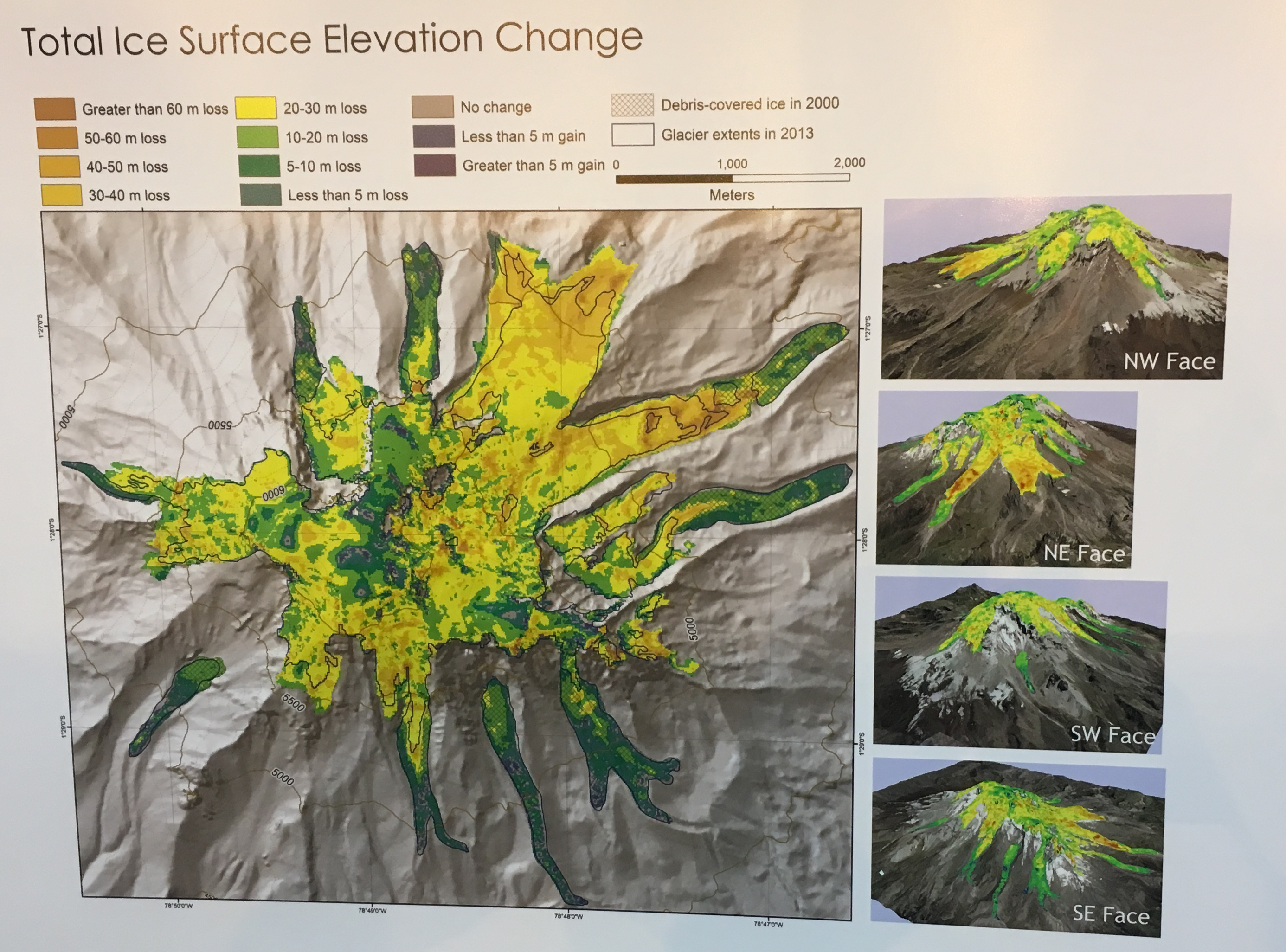
Jeff La Freniere at Gustavus Adolphus College used several new technologies,  aerial and terrestrial LIDAR and structure-from-motion photogrammetry from drones make mass balance measurements using geodetic approaches increasingly feasible in remote mountain locations like Volcán Chimborazo, Ecuador. The result combined with a unique, 5-meter resolution digital elevation model derived from 1997 aerial imagery, reveal the magnitude and spatial patterns of mass balance behavior over the past two decades. Above are the results they found more specifically that on the Hans Meyer Glacier terminus, the mean surface elevation change since 1997 has been nearly 3 m yr-1, while on the lower-elevation Reschreiter Glacier the mean elevation change has been approximately 1 m yr-1 .

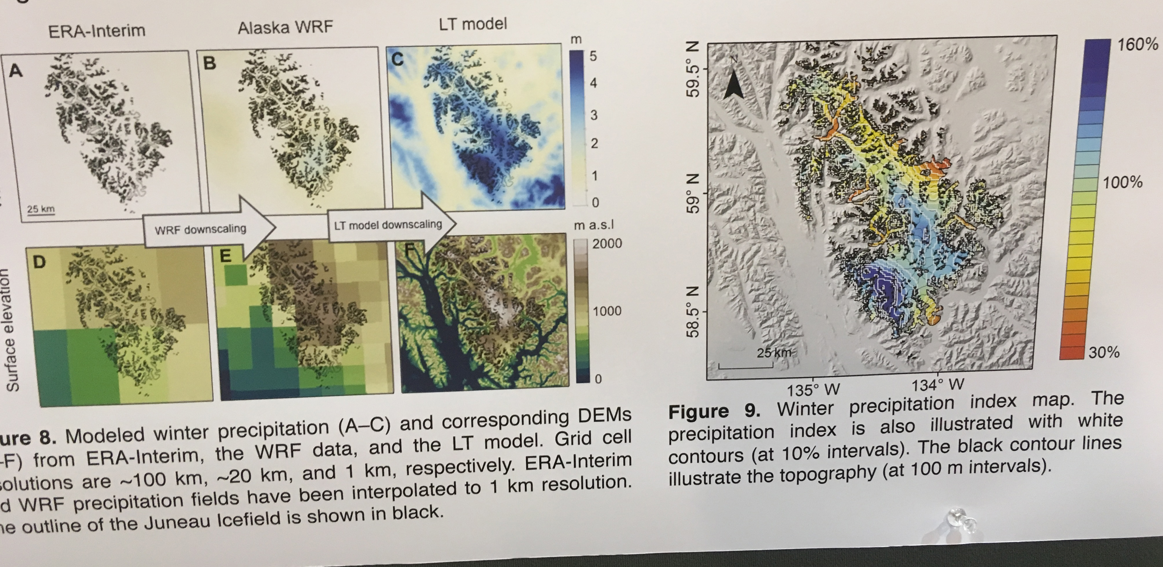
Aurora Roth, University of Alaska Fairbanks  developed and applied a linear theory of orographic precipitation model to downscale precipitation to the Juneau Icefield region over the period 1979-2013. This LT model is a unique parameterization that requires knowing the snow fall speed and rain fall speed as tuning parameters to calculate cloud time delay. The downscaled precipitation pattern produced by the LT model captures the orographic precipitation pattern absent from the coarse resolution WRF and ERA-Interim precipitation fields. Key glaciological observations were used to calibrate the LT model. The results of the reference run showed reasonable agreement with the available glaciological measurements, which is what glacier mass balance observations have shown. The precipitation pattern produced was consistent regardless of horizontal resolution, and climate input data, but the precipitation amount varied strongly with these factors.  The import is to help model mass loss from glaciers in Southeast Alaska which will alter downstream ecological systems as runoff patterns change. 

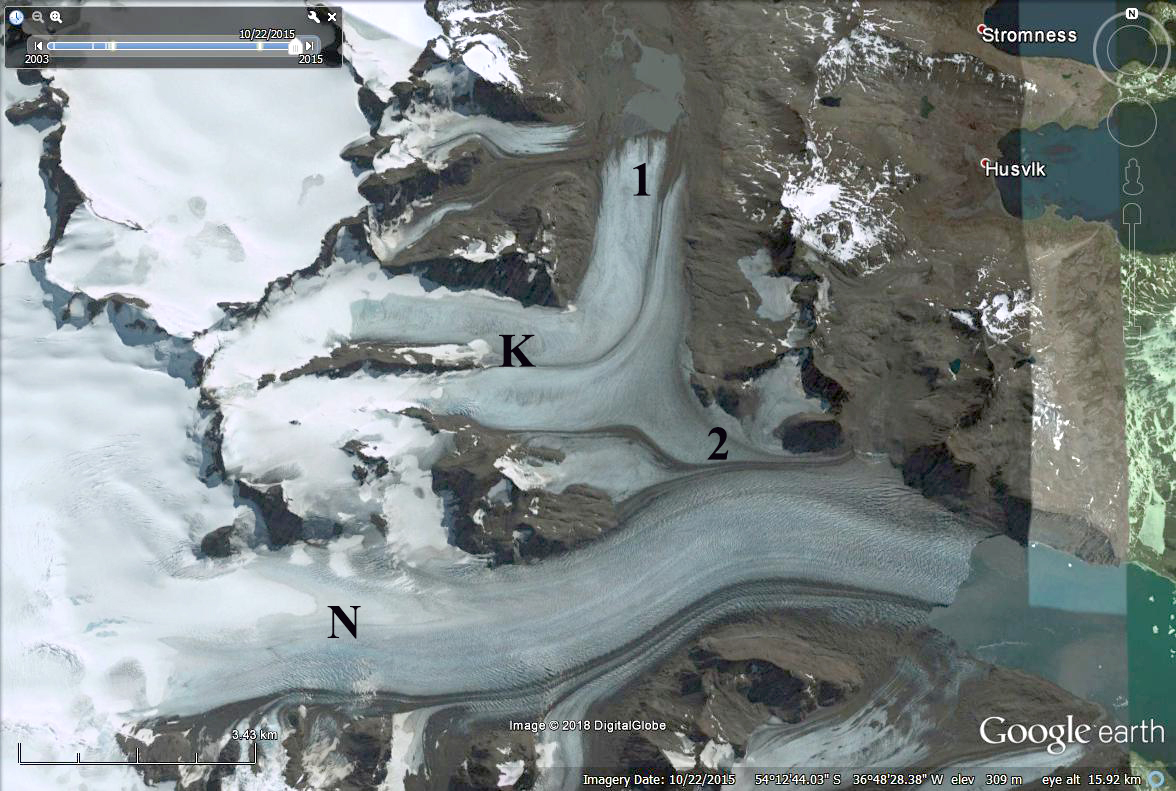
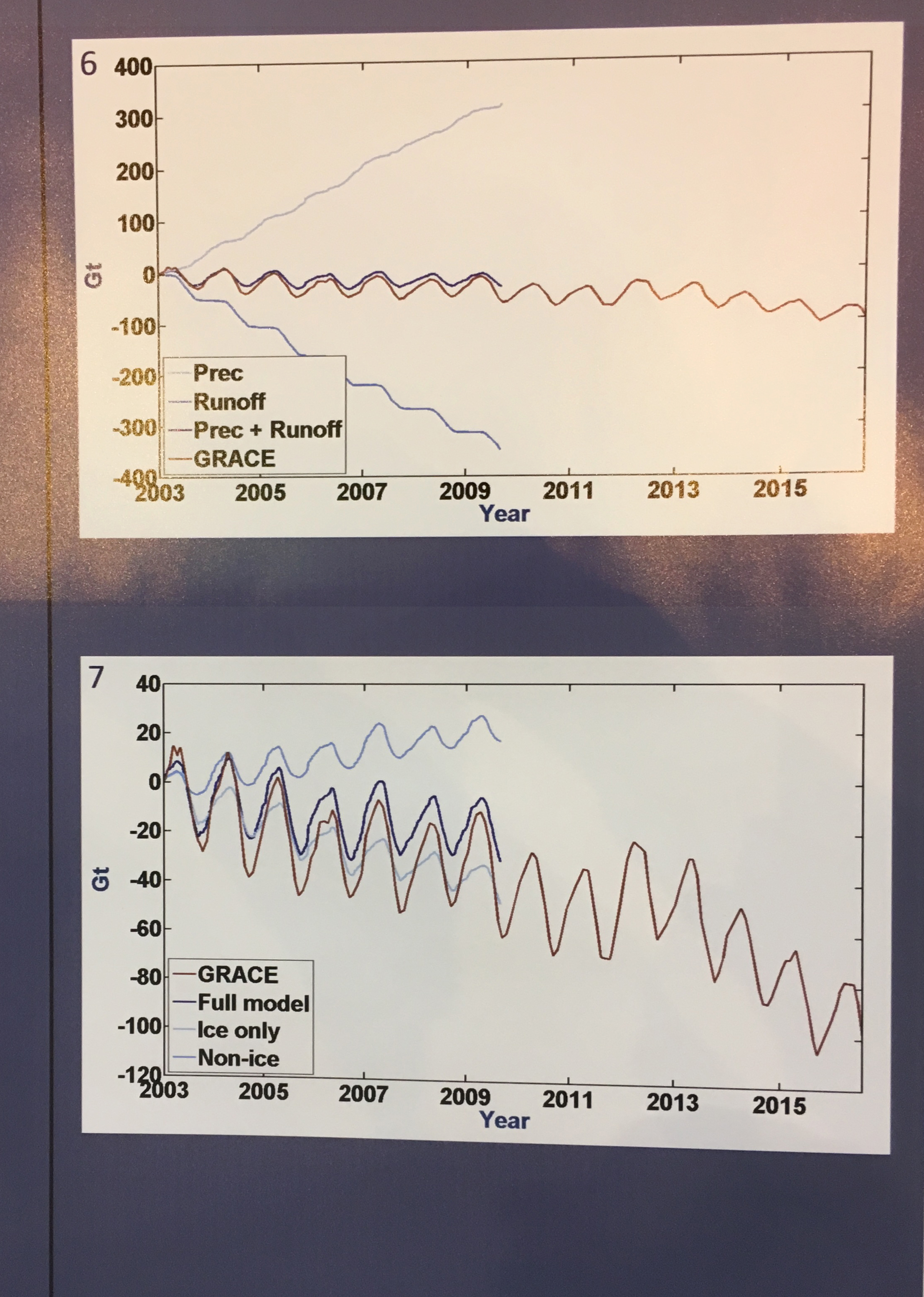
Joanna Young, University of Alaska Fairbanks  focuses on partitioning GRACE glacier mass changes from terrestrial water storage changes both seasonally and in long-term trends using the Juneau Icefield, which has long term glacier mass balance data, as a case study for . They leverage the modeling tool SnowModel to generate a time series of mass changes using assimilated field observations and airborne laser altimetry, and  compare to GRACE solution from the NASA Goddard Space Flight Center Geodesy Laboratory .  This is one of the first to analyze GRACE at the sub-mountain range scale, and to examine terrestrial water storage trends at a smaller scale than the full Gulf of Alaska. The figure above looks at subannual and long-term changes of the Juneau Icefield from 2003 to present.

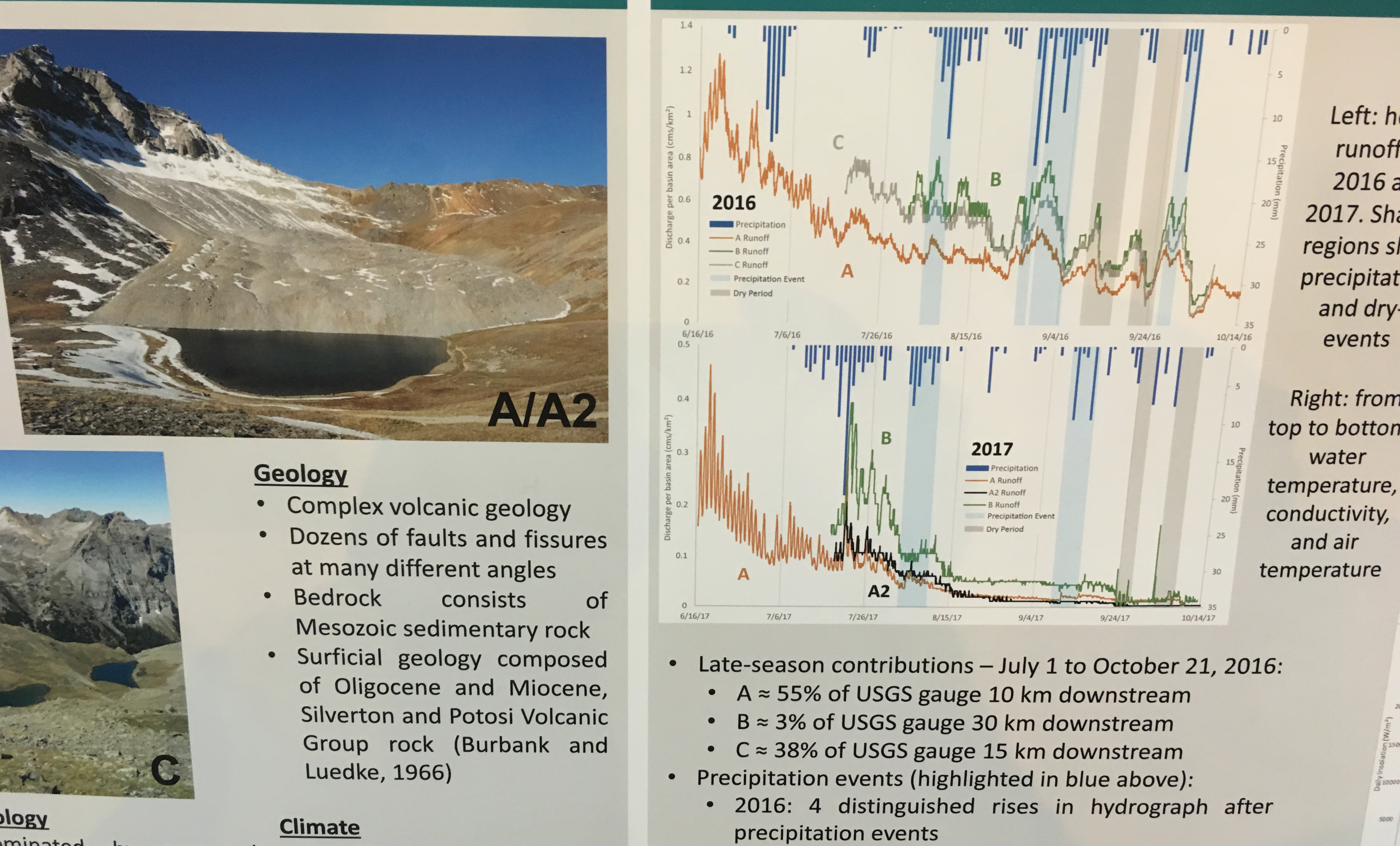
Emilio Ian Mateo, University of Denver  Looked at rock glaciers in the San Juan Mountains of Colorado examining how slope aspect and rising air temperatures influenced the hydrological processes of streams below rock glaciers. Detailed findings  illustrated above from 2016 and 2017 show that air temperature significantly influenced stream discharge below each rock glacier. Discharge and air temperature patterns indicate an air temperature threshold during late summer when rock glacier melt increased at a greater rate. The results suggest that slope aspect influences stream discharge, but temperature and precipitation are likely the most components of the melt regimes. 

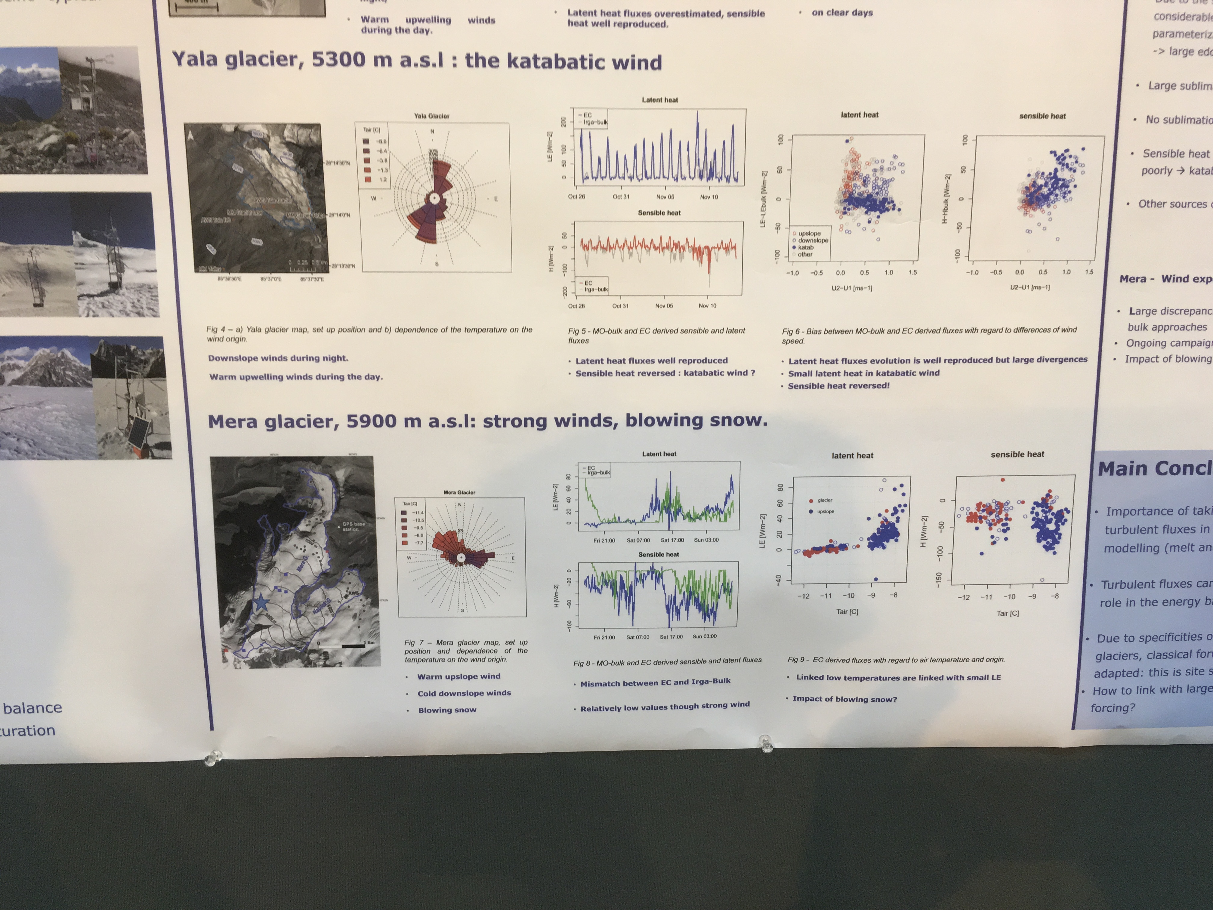
Maxime Litt, Utrecht University installed an eddy-correlation system (Campbell IRGASON) during a period of 15 days over the Lirung glacier in the Langtang Valley in Nepal , during the transition period between the monsoon and the dry season to examine surface energy balance.  Results are also reported from Mera Glacier and Yala Glacier. At Lirung Glacier during the day, moderate winds blow up-valley and the atmospheric surface layer is unstable. Latent (sensible) heat fluxes scale between 50 and 150 (50 and 250) Wm– 2 during the day, thus drying and cooling the debris and significantly impact SEB. At night, weak down-glacier winds are observed and fluxes remain weak. Yala and Mera Glacier are different environments and illustrate the variations in position on SEB.

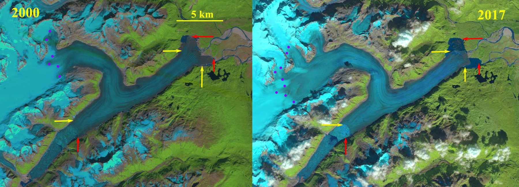
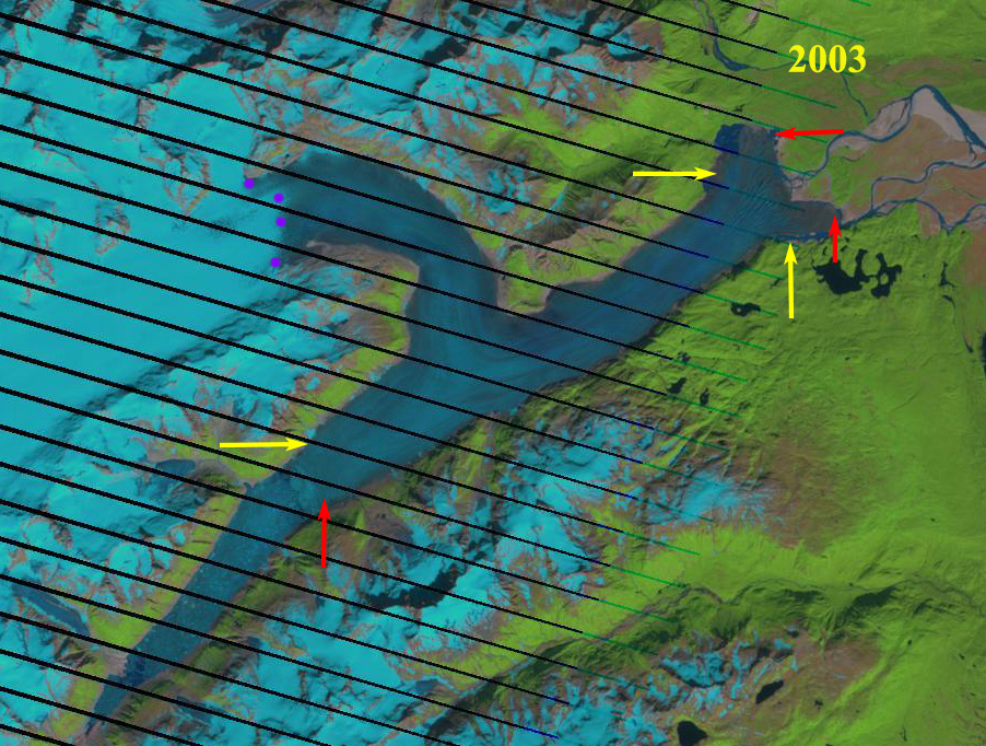
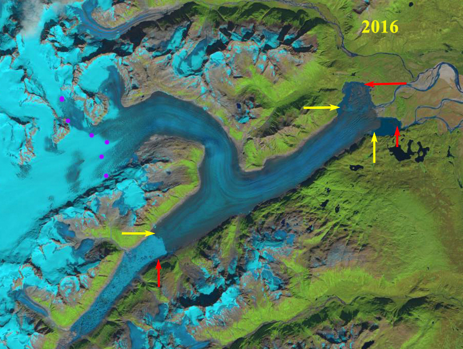
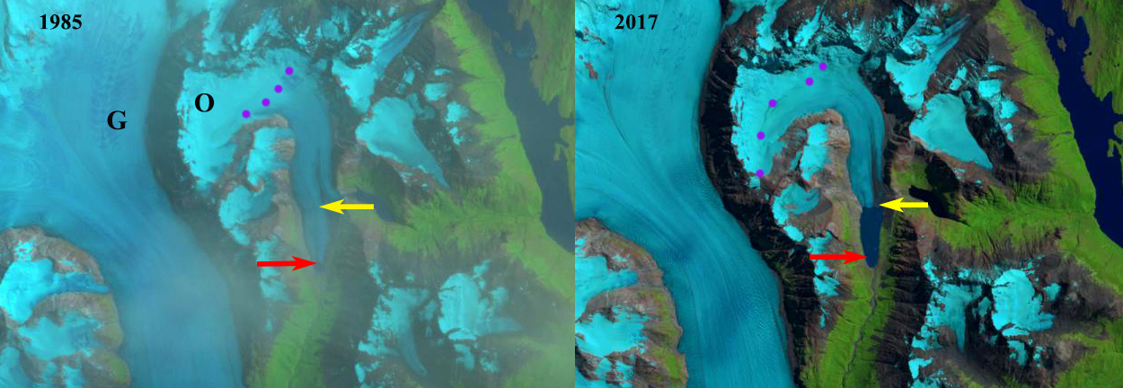
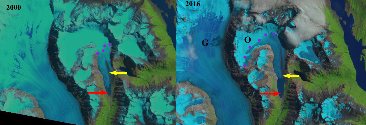
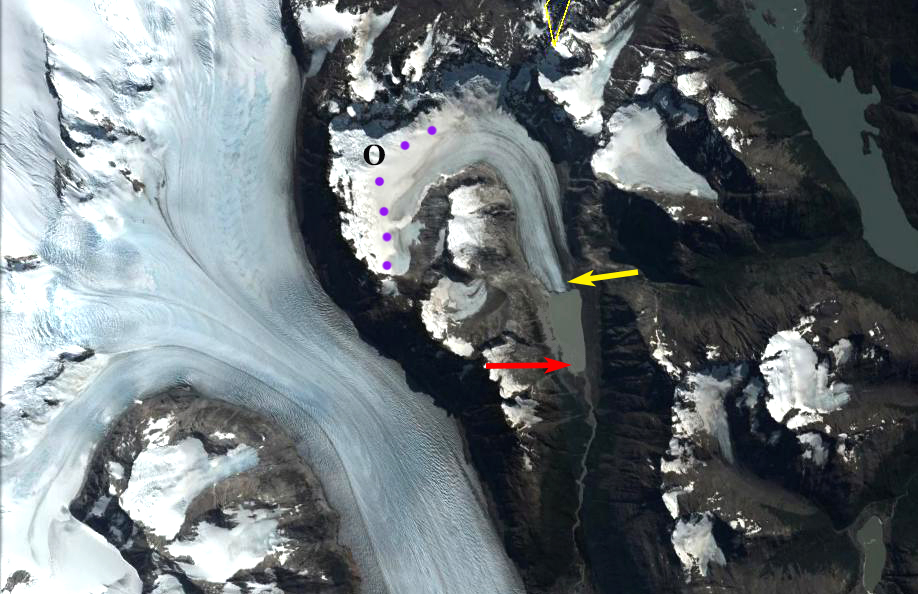
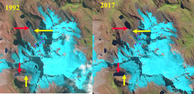
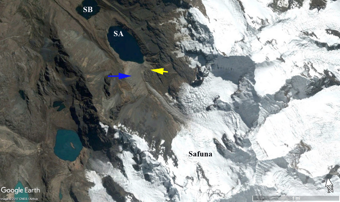
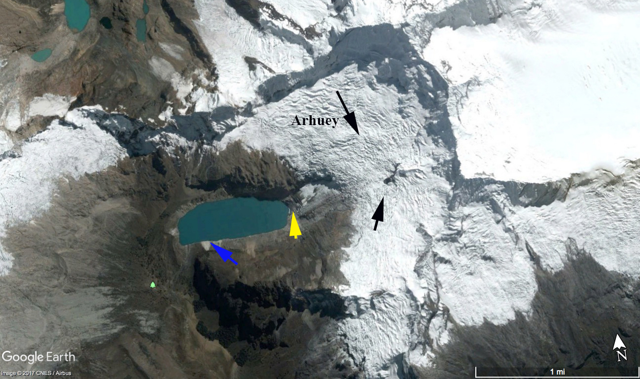
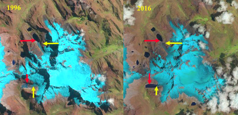
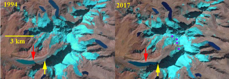
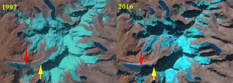
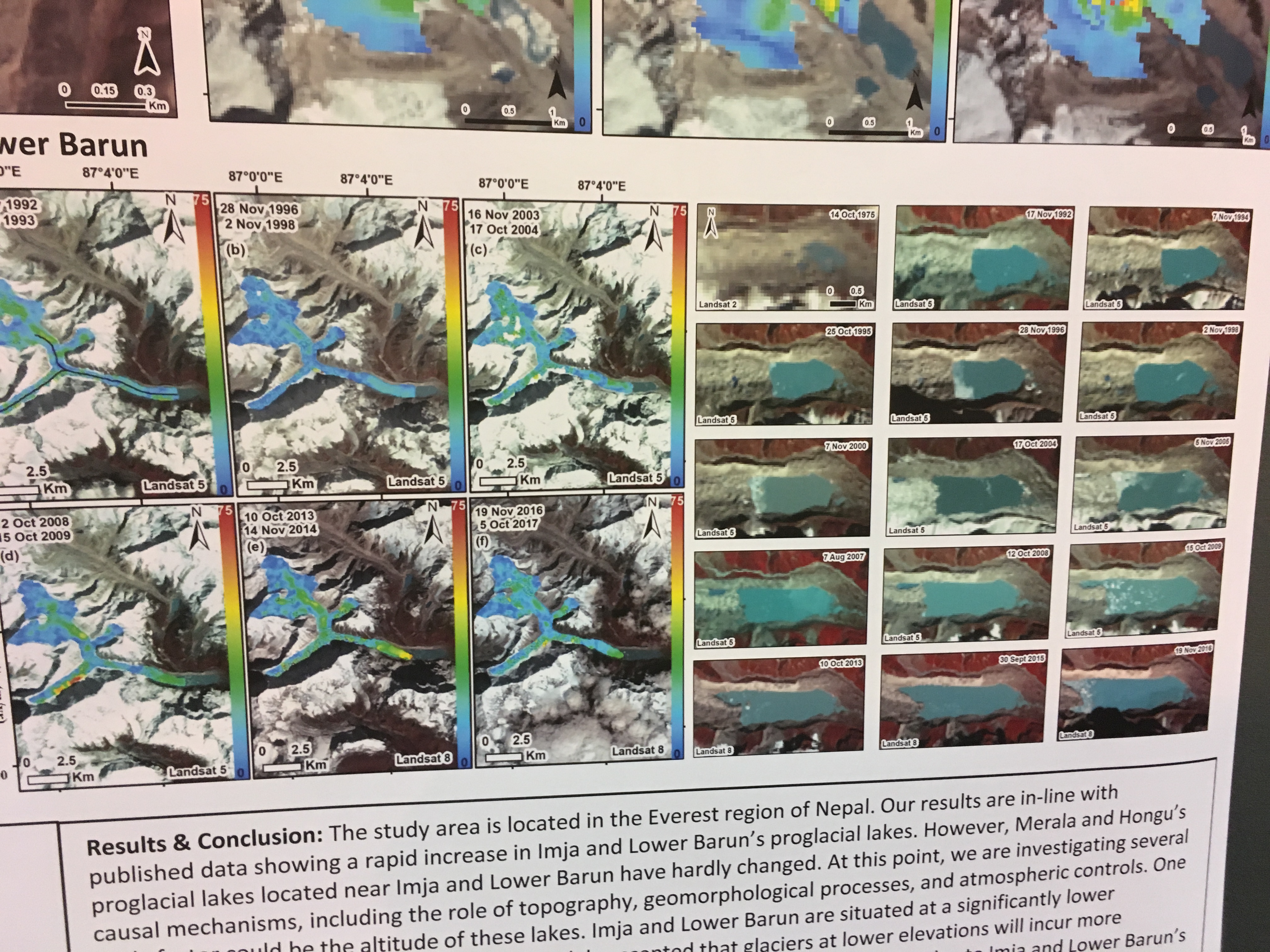
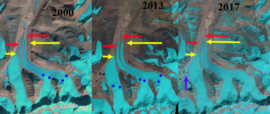
Katherine Strattman, University of Dayton reported on a study of the  Imja, Lower Barun, and Thulagi Glaciers in the Nepal Himalaya. The retreat of the glaciers has led to proglacial lakes continuing to dramatically increase in area. They used Landsat, ASTER, and Sentinel satellite imagery to study the conditions of these glaciers. They assessed interannual changes in surface ice velocity from the early 1990s to present. They found both long-term and short-term velocity variations.  Satellite imagery indicates the three lakes exhibit three contrasting trends of lake growth: Imja Lake has a strong accelerating growth history since the 1960s, Lower Barun a very slow accelerating growth, and Thulagi a decelerating growth, even as the glaciers of all three lakes have thinned. Above is the velocity of Barun Glacier showing velocity changes and growth of the lake.

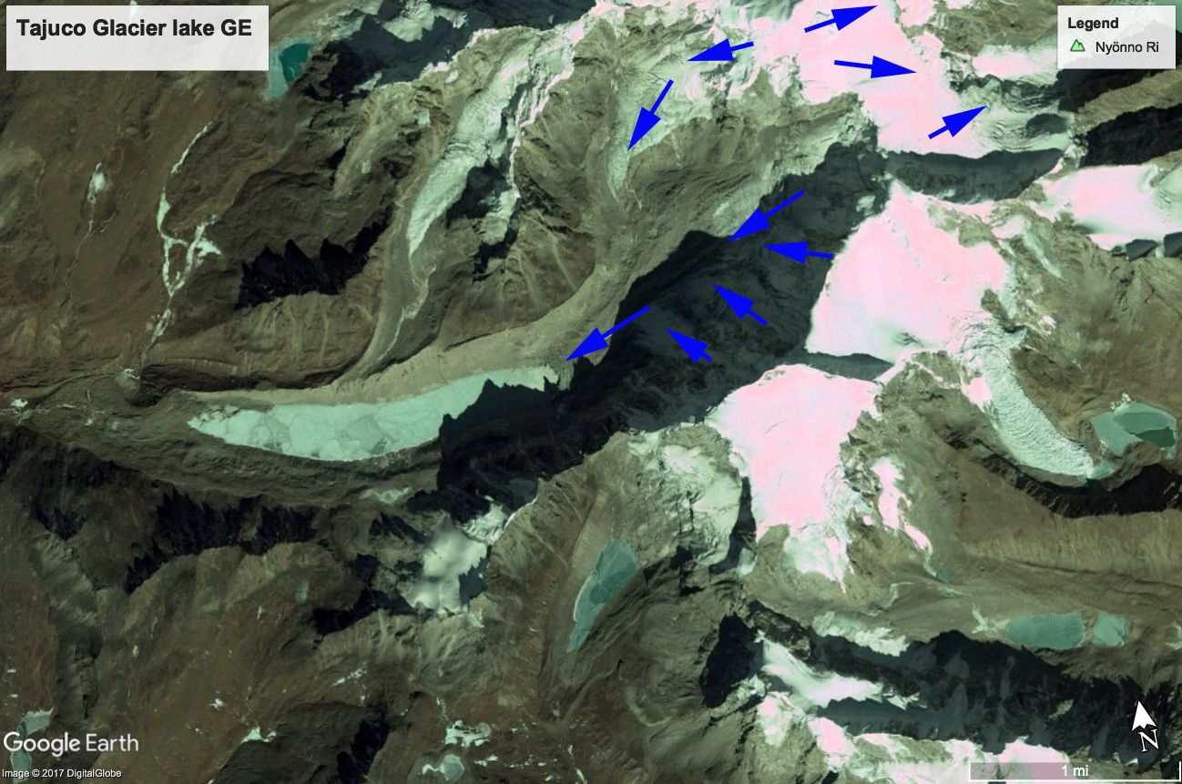
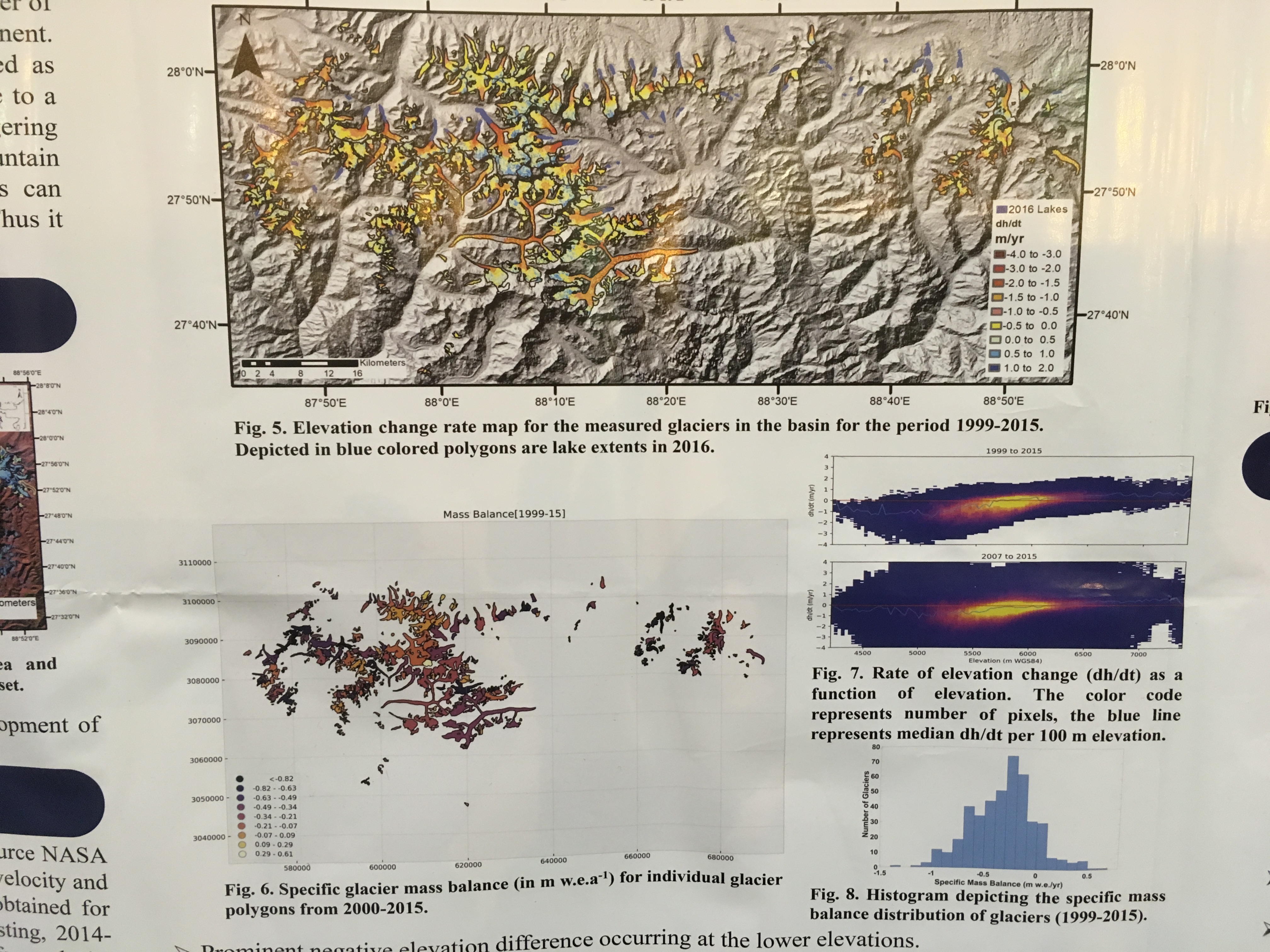
Shashank Bhushan, Indian Institute of Technology Dhanbad developed a hazard assessment of  moraine dammed glacial lakes in Sikkim Himalayas. They generated high-resolution DEMs using the open-source NASA Ames Stereo Pipeline (ASP) and other open-source tools to calculate surface velocity and patterns of glacier downwasting over time. Geodetic glacier mass balance was obtained for three periods using high-resolution WorldView/GeoEye stereo DEMs, Cartosat-1 stereo DEMs and SRTM. Initial results revealed a region-wide negative annual mass balance of -0.31± m w.eq. for the 2007-2015 period. 

From a Glaciologists Perspective AGU Day 2

It has been 30 years since my first experience at the AGU, at that time glaciology and the cryosphere played a small role.  Today that is clearly not the case.  Today just a glimpse of a few of the many interesting glaciers studies are provided to again illustrate the vast array and amazing detail of work being conducted.

Samiah Mustafa, Brown University presented research looking at the ability of a melt model to generate accurate discharge at three watersheds in West Greenland; North River (Thule), Watson River (Kangerlussuaq), and Naujat Kuat River (Nuuk). In each watershed they modeled melt at daily, 5, 10 and 20 day time scales.  They found Nuuk and Thule basins did not do well at a daily time scale, but do capture variability over 5-, 10-, and 20-day means (r2 > 0.7). Results at Watson River were in good agreement at each time scale. Model agreement with river flow data  is reduced during periods of peak discharge, particularly for the exceptional melt and discharge events of July 2012 evident in chart above.

Waldemar Walczowski, Institute of Oceanology Polish Academy of Sciences reported on a study combining glacier retreat and examination of water temperatures in the Hornsund fjord (southern Svalbard), collected under the Polish-Norwegian projects GLAERE and AWAKE-2.  The observed direct contact of warm oceanic water with a glacier’s calving face enhances submarine melting, undercutting and glacier calving.  The turbulent plumes of subglacial meltwater were key in heat transfer and influence glacier retreat. 

Martin Wearing from Lamont Doherty examined the development of crevasses in the past as the Ronne Ice Shelf advanced over the Henry Ice Rise.  The ice shelf thickened and advanced coming in contact with the bedrock high and generating crevasses that first formed around 600o years ago.  They discovered the featured in radar profiles of the ice shelf.  The sequence of crevasse development is seen above.

Morgan Whitcomb from University of Michigan used a simple damage evolution law, based on crevasse distributions as a continuum field to yield estimates of ice shelf calving rates when combined with the Community Ice Sheet Model (CISM).  Their basal melt function enhanced crevasse growth near the ice shelf terminus, leading to increased iceberg calving.  The diagram above shows the model predicts broadly correct calving rates for ice tongues ranging in length from 10 km  on Erebus to over 100 km  on Drygalski Glacier.


Ann Hill, Skidmore college working with the Juneau Icefield Research Programs velocity monitoring program reports on a comparison of velocity and surface elevation on Taku Glacier from 1997-2017.  The velocity on the main profile was consistent, as it had been back to 1950.  The surface elevation has experienced thinning after 1997 after a prolonged period of thickening.  Above are three velocity profiles with red and blue arrows from 1997 and 2017 mostly overlaying each other because velocity did not change.  Above are profiles of height changes for various periods.

 Lu An from UCal Irvine used multiple sources to reconstruct bathymetry glacier bed topography near the grounding line of Sermeq Avangnardleq (AVA) and Sermeq Kujatdleq (KUJ) in central West Greenland.  They used high resolution airborne gravity data from AIRGrav and MultiBeam Echo Sounding data collected in the fjord. The seamless topography obtained across the grounding line reveal the presence of a 300-m sill for AVA that has stabilized its terminus.  For KUJ shown above the sill has helped stabilize the glacier though it has still retreated ~1 km and has led to iceberg stranding.

From a Glaciologists Perspective AGU Day 1

The theme changes from a glaciers to a glaciologists perspective with a focus on selected work at the AGU 2017. The research discussed here is from the Poster Paper sessions the most interactive part of the convention.  The following are some interesting snapshots of the breadth and depth of ongoing research.  The most compelling figure from each poster is used.

Richard Forster, U of Utah team presented work on the firn aquifer in Greenland.  A feature we did not even know existed until 2011. They have conducted four field seasons,  using ground penetrating radar  and magnetic resonance soundings to map water table elevation, thickness and volume in several areas.  They found the aquifer thickness has a typical thickness of 10-30 m.  Further they found that firn aquifers have existed since at least 1993 and have expanded and shifted with time see above image.

Kristin Poinar, NASA GSFC team examined the drainage of supraglacial lakes in Greenland. They investigated factors that control when and where the lakes drain to the ice sheet base. They observed  359 lake drainage events in a west Greenland region and compare the dates of these drainage events to strain rates calculated from satellite data. They noted both slow draining and fast draining lakes, the faster drainages occurring later in the summer on average. They found that strain rates did not satisfactorily predict lake drainage date.  

Vena Chu at UC-Santa Barbara’s team mapped river networks On Russell Glacier that terminate into moulins which connect surface melt to englacial and subglacial drainage networks. They used WorldView imagery to show development of molins and their migration between 2012 and 2015.   The majority of moulins they mapped in 2015 were  moulins in 2012. New moulins most commonly formed in crevassed, thinner ice areas near the ice margin, and a lesser but significant quantity at higher elevations above 1300 m.

Rohi Muthyala, Rutgers University team measured the discharge of supraglacial streams for three months, constructing rating curves.  They compared air temperature and discharge in the upper and lower basin.  The upper basin was more related to the daily air temperature. The stream system feeds into a moulin system.

Mariah Radue, University of Maine’s team mapped and dated the moraines and erratics adjacent to Potanin Glacier in the Mongolian Altai (49°N, 88°E). They used 10Be surface-exposure chronology to date glacial landforms mapped using satellite and Drone imagery. Based on our glacial reconstruction, we estimate changes in atmospheric temperature from the Last Glacial Maximum to the Late Holocene using snowline reconstruction techniques. Mongolia is a unique location because it is isolated from oceanic influences and a climate could provide insight into the roles of local radiation forcing from earth orbital changes, greenhouse gases, and a Asian climate dynamics.

Konstanz Haubner, with a team from GEUS in Denmark provided a model simulating velocity and ice thickness change at Upernavik Glacier, Greenland from 1849-2017. In the image above the retreat is illustrated, separating into three separate glaciers with a more bedrock pinning points to stabilize.  They noted  a changing contribution to Upernavik’s ice mass loss from surface melt and ice dynamics in different time periods.


Muller Ice Shelf, Antarctica Retreat and Rift Zone Expansion

Muller Ice Shelf (M) in 1989 and 2017 Landsat images fed by the Antevs (A) and Bruckner Glacier (B). The ice front is shown with yellow dots with separate calving margins on either side of Humphrey Island (H).  The blue arrow indicates a developing rifted zone of melange ice.  The pink arrows point out icebergs among sea ice. 

Muller Ice Shelf is on the west side of the Antarctic Peninsula and  is one of the smallest remaining ice shelves covering 40 km2 in 2007.
It is the northernmost ice shelf on the western side of the Peninsula and is fed by Bruckner Glacier (b) and Antevs Glacier (A), and is pinned on Humphreys Island (H). The glacier advanced from 1947 to 1956 with subsequent retreat until  another advance period from 1974-1986 when the ice front advance led to a 4 square kilometer expansion Cook and Vaughan (2010).  Retreat has since ensued Domack et al. (1995) suggesting that warm CDW that is currently within the fjord may be contributing to the rapid bottom melting and retreat of the ice-shelf  in recent years.    Here we use Landsat imagery to identify changes from 1989 to 2017.  

In 1989 the western side of the ice shelf edge is near the north end of Humphrey Island and the east margin near a cape half along the eastern edge of Humphrey Island.  By 2001 the western margin has retreated 1.5 km and the eastern margin 1.2 km.  In 2016 the both the eastern and western margin have retreated to the southern end of Humphrey Island.  The island still acts as a pinning point, but this connection is becoming tenuous.  Of equal importance is the development of an area of substantial rifting north of the bluff on the southern margin of the ice shelf between Antevs and Bruckner Glacier at the blue arrow. In 2017 the rifting has further expanded, the ice melange now covering an area of ~1 square kilometer.  From 1989 to  2017 the western margin has retreated 2.5 km and the eastern margin 1.5 km.  The retreat due to calving is ongoing as indicated by the number of new icebergs in the Feb. 2017 image, pink arrows. Between this area of rifting and the decrease in connection to Humphrey Island the Muller Ice Shelf is poised for rapid disintegration like nearby Jones Ice ShelfBethan Davies provides a detailed look at the weaknesses of other Antarctic Peninsula ice shelves.

Muller Ice Shelf (M) in 2001and 2016 Landsat images fed by the Antevs (A) and Bruckner Glacier (B). The ice front is shown with yellow dots with separate calving margins on either side of Humphrey Island (H).  The blue arrow indicates a developing rifted zone of ice weakness. 

Google Earth image from 1998 and 2016 indicating rift development at blue arrow. 

Figure 4.1 from Cook and Vaughan (2010)   illustrating changes in ice shelf area.

Zhongni Glacier Retreat, China and Hydropower

Zhongni Glacier changes from in Landsat images from 1994 to 2015. The red arrow is the 1994 terminus, yellow arrow the 2015 terminus, purple dots the snowline and purple arrows lakes adjacent to the margin of the western glacier in 1994.

Zhongni Glacier is 15 km northwest of Gangotri Glacier just across the border into China.  The glacier drains in to the Langgen Zangbo, which becomes the Sutlej River in India. The Sutlej River has a 1000 MW  Karcham Wangtoo hydropower plant and a 300 MW Baspa hydropower plant (see below). 

The glacier is comprised of three main tributaries separated by two prominent medial moraines.  The width of the medial moraine extending to the main terminus is over 200 m. Here we use Landsat imagery to identify the glacier changes from 1994 to 2017.

The western tributary acts as a separate glacier and in 1994 has several adjacent small melt lakes, purple arrow terminating with a narrow band of ice at the red arrow.  The snowline is at ~5900 m.  The eastern two tributaries extends 700 m  further downvalley before terminating. In 2000, there has been retreat of 100-200 m of the western tributary and main glacier, and the snowline is at 5750 m.  In 2013 the snowline is at 5800 m.  In 2015 the snowline is at 5750 m.  By 2015 the western tributary margin has receded from the lakes at the purple arrow. The snowline in 2015 is at 5750 m.  In each case the images are far from the fall and the snowline during the post-monsoon season is not the highest elevation.  In 2017 there is new snowfall in late November obscuring the snowline.  Overall retreat from 1994-2015 of the eastern tributary has been 500 m and of the western tributary 900 m.  The western tributary has also lost 200 m of width at the purple arrow. On nearby Gangotri Glacier, India it has been observed that the ablation season has been extending through fall into early winter. The retreat is less pronounced than glaciers terminating in pro-glacial lakes such as Chutanjima Glacier

Zhongni Glacier changes from in Landsat images of 2000, 2013 and 2017. The red arrow is the 1994 terminus, yellow arrow the 2015 terminus, purple dots the snowline and purple arrows lakes adjacent to the margin of the western glacier in 1994.

Zhongni Glacier in 2012 with the snowline at 5900 m in Digital Glacier imagery. Purple arrows indicate medial moraines.

The Karcham Wangtoo Hydropower (lower yellow arrow) and Baspa Hydropwer station (upper yellow arrow) which both have small reservoirs.

Global Glacier Change Bulletin-Many Glaciers Same Story


Cumulative glacier mass balance losses reported by WGMS by region, all glacier, reference glaciers and geodetic mass balance (Sholes Glacier, WA in background).  The data set size, location and type changes but the story remains the same, mass loss resulting from global temperature increase.

The World Glacier Monitoring Service has released the second bulletin of Global Glacier Change.  The bulletin provides detailed global and regional information on alpine glaciers particularly for 2014 and 2015.  There is data reported from 621 glaciers.  The glaciers vary in type and location, yet their response is the same retreat and mass balance loss as a result of the global temperature increases.  There are currently 41 reference glaciers with at least 30 consecutive years of detailed field measurement of mass balance.  Additionally mass balance is typically reported from 60-80 other glaciers.  The graph below indicates that the reference glacier network mass balance losses parallels the losses of all glaciers and that of geodetic assessment of mass loss from remapping.  The report indicates that alpine glaciers have lost 0.9 m w.e. per year.  This continues the unprecedented trend of mass loss that is driving glacier retreat as well. In 2014 and 2015 316 mass balance observations are reported from 166 glaciers.  There are 889 terminus change observations reported from 528 glaciers. The results in graph after graph illustrate that glaciers in all regions of the globe are experiencing mass loss and retreat.  As the United States representative to the WGMS, helping pull together each strand of data, is a key task.  The result unfortunately is a very strong line of data built of all these strands of glaciers losing mass.  The report also contains preliminary data from 2016, which was the 37th consecutive year of mass loss as reported in BAMS State of the Climate 2016 (Pelto, 2017).  The deadline for posting initial results on mass balance for reference glaciers in 2017 was Dec. 1 2017.  Reporting on the US glaciers it is clear that 2017 will be another year of substantial losses in this region. 


Annual glacier mass balance reported for each region.  The coloration indicates the increase in mass balance loss in each region with global temperature increase. 

There is a section of the bulletin on each region including graphs of terminus change and mass balance on selected glaciers. Below are examples from Western North America and Central Europe.  For reference glaciers data is submitted that includes maps of the mass balance, and then charts are derived from WGMS illustrating mass balance changes and the relationships between mass balance and the equilibrium line altitude, and between mass balance and the accumulation area ratio.  


Alsek Glacier, Alaska Retreat & Glacier Separation

Alsek Glacier in a 1984 Landsat image and 2017 Sentinel image.  Red arrows indicate 1984 terminus, yellow arrows 2017 terminus location, pink arrows tributaries that joined the glacier in 1984 and purple dots the snowline.  AR=Alsek River, G=Gateway Knob and P=Prow Knob.

Alsek Glacier descends from the Fairweather Range terminating in Alsek Lake on the coastal plain. The glacier terminated at Gateway Knob (G) near the outlet of Alsek River from Alsek Lake in the early part of the 20th century (Molnia, 2005). At that time it had a joint terminus with Grand Plateau Glacier. The glacier retreated 5-6 km by 1984 along the central margin from Gateway Knob. The glacier remained connected with the Grand Plateau Glacier in 1984. In 1960 the glacier had a single terminus joining downstream of an unnamed island in Alsek Lake, that Austin Post told me reminded him of a boats prow. This “Prow Knob” (P) much like Gateway Knob a century ago stabilizes the terminus. Retreat from this knob will lead to an increase in retreat of Alsek Glacier. Here we examine the change from 1984-2017 with Landsat and Sentinel imagery.

In 1984 the terminus location is denoted with red arrows it has separated into two termini on either side of “Prow Knob”. The northern terminus tongue is located on a narrow island on the north side of Alsek Lake. The southern tongue merges with the northern arm of Grand Plateau Glacier. Two tributaries at the pink arrows merge with the main glacier. In 1984 the snowline is at 900 m. By 1999 the northern tongue has retreated from the narrow island, which exposes the terminus to enhanced calving. The southern terminus has separated from the Grand Plateau Glacier. In 1999 the snowline is at 900 m. By 2013 the northern terminus has retreated almost to the northern end of “Prow Knob” and the southern terminus is directly south of “Prow Knob” in a 1.8 km wide channel. By 2016 two tributaries of Alsek Glacier are fully detached from the glacier, pink arrows. In 2017 the northern terminus tongue has retreated 3.7 km since 1984 into the 2.0 km wide channel on the northeast side of “Prow Knob”. The center of the southern terminus has retreated 3.0 km since 1984 and remains in the channel on the south side of “Prow Knob”. The length of the calving front has declined from an 8 km long calving front in 1984 to a 4 km calving front in 2017. In both 2016 and 2017 the snowline is at 1200 m, at this elevation the mass balance of the glacier will be significantly negative driving further retreat. Larsen et al (2007) indicate thinning in the lower Alsek Glacier of 3+m/year in the last half of the 20th century, indicating the glacier is a in a long term adjustment to climate change.  The retreat of this glacier is similar to that of Walker Glacier and North Alsek Glacier, and less than that of the northern arm Grand Plateau Glacier to which it was connected in 1984 or Yakutat Glacier a short distance north.   

Alsek Glacier in a 1999 Landsat image .  Red arrows indicate 1984 terminus, yellow arrows 2017 terminus location, pink arrows tributaries that joined the glacier in 1984 and purple dots the snowline.   P=Prow Knob.

Alsek Glacier in 2014 Google Earth Image,indicating flow directions. 

Alsek Glacier in a 2016 Landsat image .  Red arrows indicate 1984 terminus, yellow arrows 2017 terminus location, pink arrows tributaries that joined the glacier in 1984 and purple dots the snowline.   P=Prow Knob.


Bridge Glacier, Southeast Alaska Retreat & Lake Formation

Bridge Glacier in Landsat image from 1984 and Sentinel image from 2017. The red arrow indicates the 1984 terminus where no lake exists, yellow arrow is 2017 terminus, orange arrows are selected tributaries and purple dots the snowline. 

Bridge Glacier drains the same icefield as the Wright and Speel Glacier 45 km southeast of Juneau, Alaska. Here we examine the changes in this glacier from 1984-2017 using Landsat and Sentinel imagery.

In 1984 the glacier ended on an outwash plain at the head of a branch of Speel River. The red arrow indicates the 1984 terminus for each image, the yellow arrow the 2017 terminus and the orange arrows three tributaries feeding the glacier.  The purple dots indicate the snowline at 1200 m. In 1984 all three tributary glaciers fed Bridge Glacier and the glacier has no proglacial lake at the terminus. In 1997 a lake basin is beginning to develop, though it is still largely filled by ice. The eastern tributary pink arrow, has lost all of its snowpack. The three tributaries at the orange arrows are connected to Bridge Glacier still and the snowline is at 1250 m. In 1999 the proglacial lake has formed and has length of 1 km, the lake has expanded south and north of the 1984 terminus position, and does not entirely represent glacier retreat.  In 2013 the glacier has retreated 1200 m from the 1984 position and the lake is still expanding. The orange arrows indicate that none of the three tributaries are still connected to the main glacier. The glacier in a sense is losing its income flow from these subsidiaries. The eastern tributary has retained some snowcover with six weeks left in the melt season in 2013, but this is mostly gone a month later, the snowline is at 1100 m. nbsp; Total retreat from 1984 to 2017 is 1900 m. In 2017 the snowline is at 1300 m, and the separation of the tributaries is by more than 500 m in each case. The snowline has been high by the end of each summer from 2014-2017 indicating retreat will continue. The retreat of this glacier is the same story as seen at nearby PattersonGilkey and Norris Glacier.

.

Bridge Glacier in Landsat images from 1997 and 2013. The red arrow indicates the 1984 terminus , yellow arrow is 2017 terminus, orange arrows are selected tributaries and purple dots the snowline. 

Bridge Glacier in USGS map when it ended on the outwash plain in 1948.