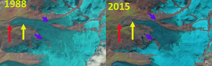
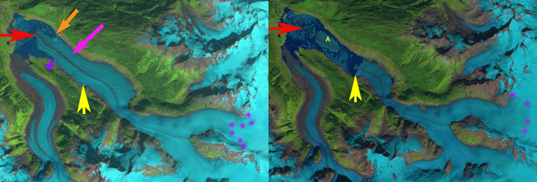
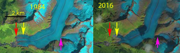
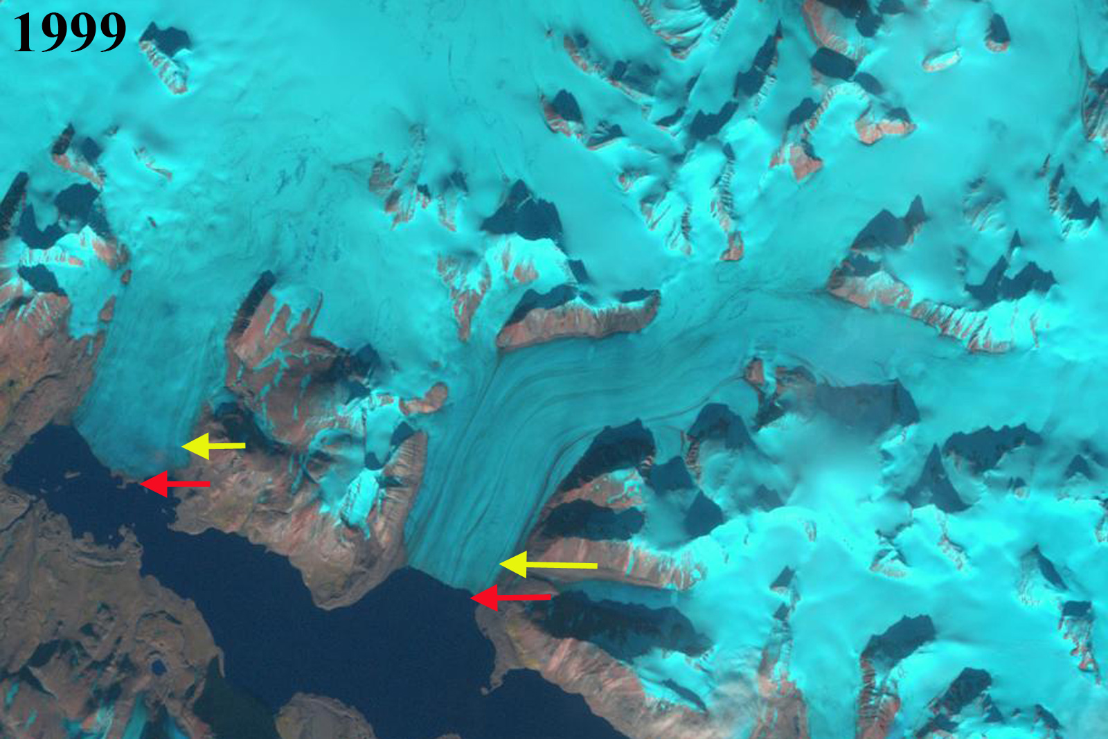
Landsat image comparison of Findelengletscher from 1988 to 2015. Red arrow indicating the 1988 terminus location and yellow arrow the 2015 terminus location. The purple arrows indicate two tributaries connected to the main glacier in 1988 and now disconnected.
Findelengletscher along with Gornergletscher drains the west side of the mountain ridge extending from Lyskamm to Monte Rosa, Cima di Jazzi and Strahlhorn in the Swiss Alps. It is the headwaters of the Matter Vispa. This glacier was also the favorite field location for David Collins, British Glaciologist/Hydrologist from University of Salford who passed away last week. David had a wit, persistence and insight that are worth remembering. This post examines both David’s findings reaching back to the 1970’s gained from a study of glaciers in this basin and changes of the glacier since 1988 as evident in Landsat images. Findelengletscher drains into the Vispa River which supports for hydropower project, with runoff diverted into two hydropower reservoirs, Mattmarksee operated by the Kraftwerke Mattmark producing 650 Gwh annually, and Lac de Dix operated by Grande Dixence that produces 2000 Gwh annually. There are two smaller run of river projects as well.
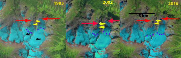
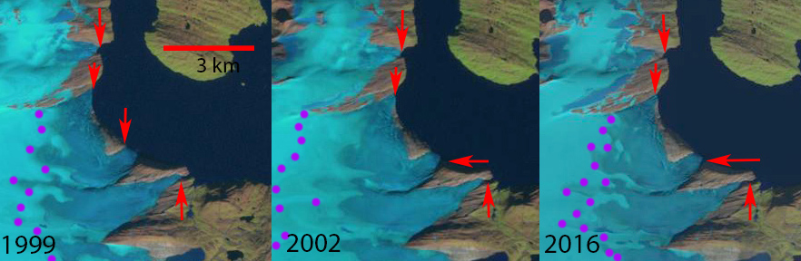
The Swiss Glacier Monitoring Network has monitored the terminus change of Findelengletscher since the 1890’s. The glacier advanced 225 m from 1979-1986, retreated 450 m from 1988-1999 and retreated 850 m from 1999-2015. This is illustrated above with the red arrow indicating the 1988 terminus location and the yellow arrow the 2015 terminus location. The purple arrows indicate two tributaries connected to the main glacier in 1988 and now disconnected. The more limited retreated from 1988-1999 is evident in images below. The retreat is driven by mass losses with Huss et al (2012) noted as 1 m/year in the alps from 2001-2011. The snowline has typically been above 3250 m too high for equilibrium in the last decade. Melt at the terminus has typically been 7-8 m (WGMS).
Collins (1979) in work funded through hydropower looked at the chemistry of glacier runoff and found that glacier meltwater emerging in the outlet stream was enriched in Calcium, Magnesium and Potassium in particular versus non-glacier runoff, this led to a much higher conductivity. Collins (1982) noted the reduction in streamflow below Gornergletscher from summer streamflow events that reduced ablation for up to a week after the event. Collins (1998) noted that a progressive rise of the transient snow line in summer increases the snow-free area, and hence the area of basin which rapidly responds to rainfall. Rainfall-induced floods are therefore most likely to be largest between mid-August and mid-September and in this period of warmer temperatures and higher snowlines. Collins (2002) Mean electrical conductivity of meltwater in 1998 was reduced by 40%. In the same 60 day period in 1998, however, solute flux was augmented by only 2% by comparison with 1979. Year-to-year climatic variations, reflected in discharge variability, strongly affect solute concentration in glacial meltwaters, but have limited impact on solute flux. Collins (2006) identified that in highly glacier covered basins, over 60%, year-to-year variations in runoff mimic mean May–September air temperature, rising in the warm 1940s, declining in the cool 1970s, and increasing by 50% during the warm dry 1990s/2000s. In basins with between 35–60% glacier cover, flow also increased into the 1980s, but declined through the 1990s/2000s. With less than 2% glacier cover, the pattern of runoff was inverse of temperature and followed precipitation, dipping in the 1940s, rising in the cool-wet late 1960s, and declining into the 1990s/2000s.. On large glaciers melting was enhanced in warm summers but reduction of overall ice area through glacier recession led to runoff in the warmest summer (2003) being lower than the previous peak discharge recorded in the second warmest year 1947. Collins (2008) examined records of discharge of rivers draining Alpine basins with between 0 and ∼70% ice cover, in the upper Aare and Rhône catchments, Switzerland, for the period 1894-2006 together with climatic data for 1866-2006 and found that glacier runoff had peaked in the late 1940s to early 1950s.
These observations have played out further with warming, retreat and more observations. Finger et al (2012) examine the impact of future warming on glacier runoff and hydropower in the region. They observe that total runoff generation for hydropower production will decrease during the 21st century by about one third due glacier retreat. This would result in a decrease in hydropower production after the middle of the 21st century to keep Mattmarksee full under current hydropower production. Farinotti et al (2011) noted that the timing of maximal annual runoff is projected to occur before 2050 in all basins and that the maximum daily discharge date is expected to occur earlier at a rate of ~4 days/decade. Farinotti et al (2016) further wondered if replacing the natural storage of glacier in the Alps could be done with more alpine storage behind dams.

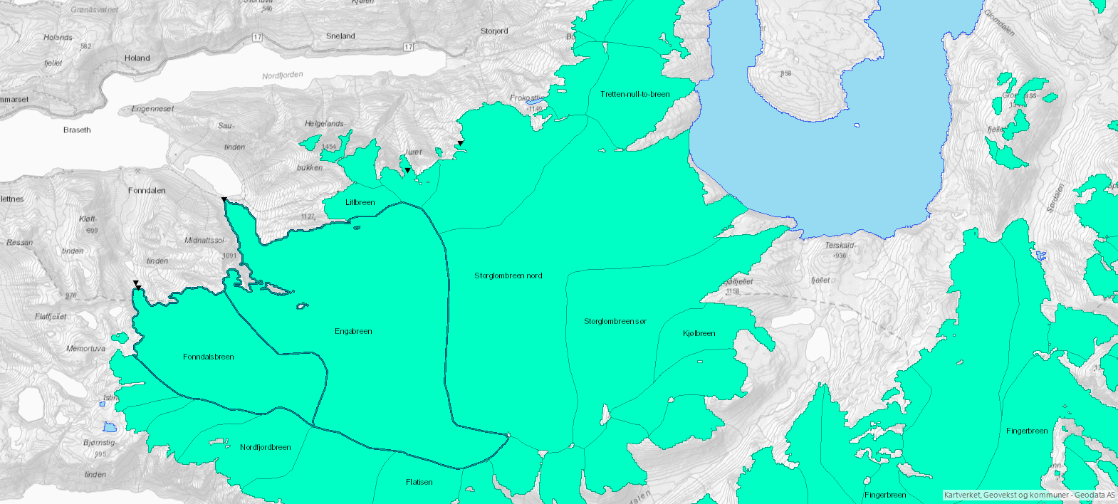
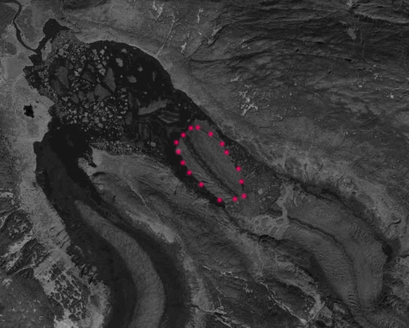
Google Earth image indicating flow of the Findelengletscher.

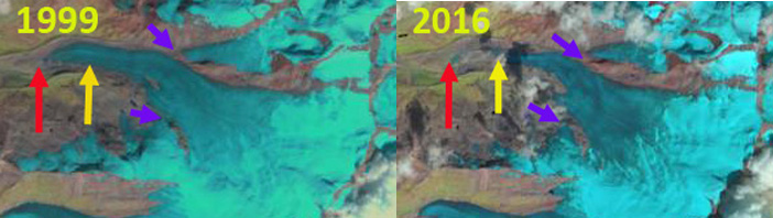
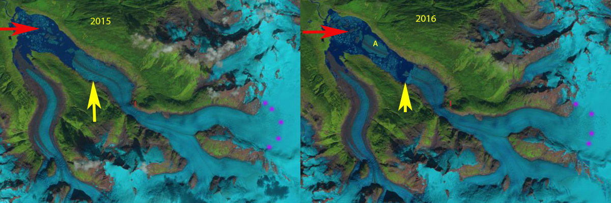
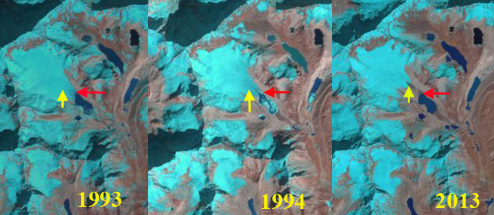
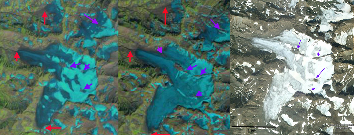
Landsat image comparison of Findelengletscher from 1999 to 2016. Red arrow indicating the 1988 terminus location and yellow arrow the 2015 terminus location. The purple arrows indicate two tributaries connected to the main glacier in 1988 and now disconnected.

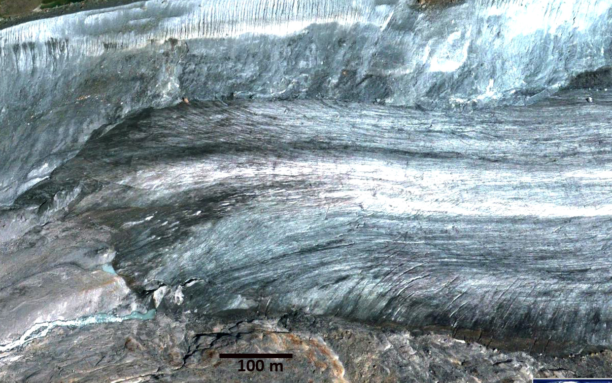
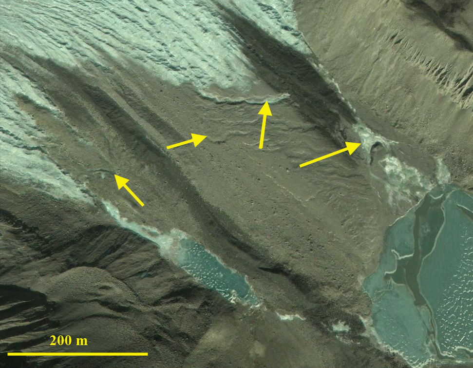
Terminus of Findelengletscher in Google Earth. The lower several hundred meters has limited crevasses, but is not particularly thin.