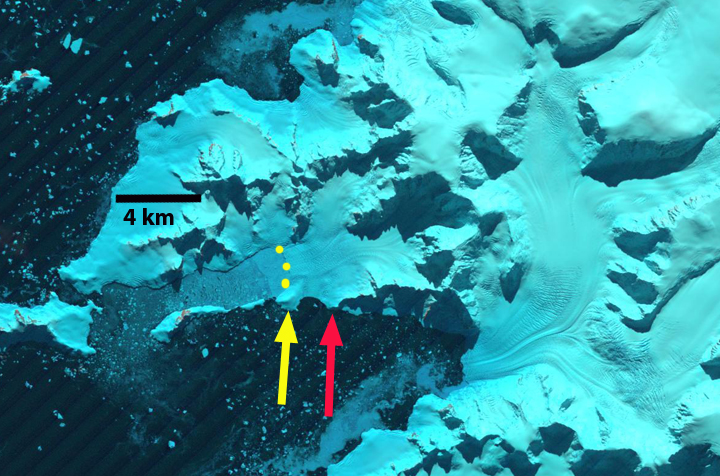
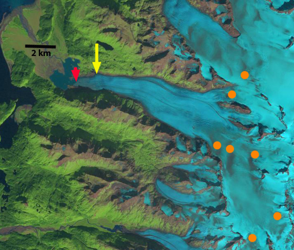
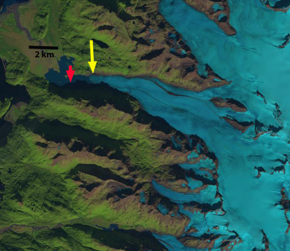
Grewingk Glacier drains west toward the Kachemak Bay, Alaska terminating in a proglacial lake in Kachemak Bay State Park. The glacier drains an icefield on the Kenai Peninsula, glaciers draining west are in the Kenai Fjords National Park. The glaciers that drain east toward are in the Kenai Fjords National Park, which has a monitoring program. Giffen et al (2008) observed the retreat of glaciers in the region. From 1950-2005 all 27 glaciers in the Kenai Icefield region examined are retreating. Giffen et al (2008)observed that Grewingk Glacier retreated 2.5 km from 1950-2005. Here we examine Landsat imagery from 1986-2014 to illustrate the retreat of the glacier. The icefront continues to calve into the expanding pro-glacial lake.
1951 based USGS Topographic map Seldovia C-3
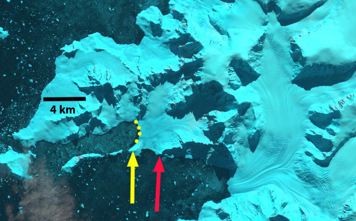
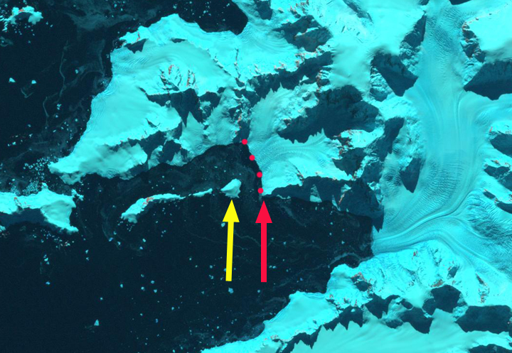
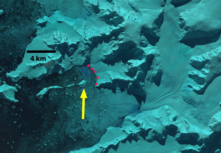
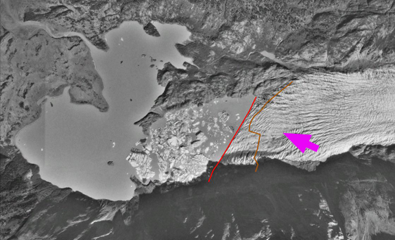
The red arrow is the 1986 terminus location at the midpoint, the yellow arrow is the 2014 mid-point terminus location. In 1951 the glacier extended beyond the peninsula at the red arrow into the wider portion of the lake. By 1986 the glacier had retreated into the narrow section of the lake extending east into the mountains, the southern margin of the terminus is further advanced than the northern margin. The orange dots indicate discoloration of the glacier surface from volcanic ash deposited on the glacier surface from Augustine Volcano in 1986. In 1989 there is not a marked change. In a 1996 Google Earth image, there is considerable icebergs indicating a recent collapse of a section of the terminus. The pink arrow indicates concentric crevasses, indicating a depression, the red line is the terminus in 1996 and the brown line the 2003 terminus.
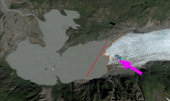
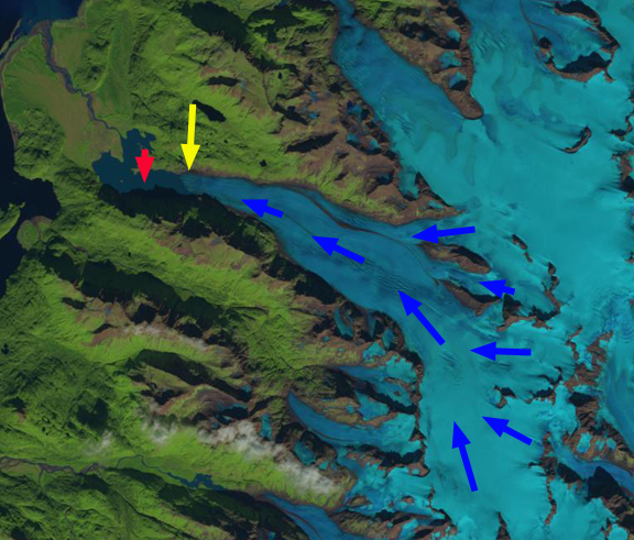
By 2001 the terminus has retreated m, and the glacier front is now oriented north-south across the lake. In 2003 the depression from 1996 now has a small supraglacial lake, the terminus has retreated 500 m on the southern margin and 200 m on the northern margin. In 2013 the glacier has retreated an additional 600 m and the southern margin has now receded further upvalley than the northern margin. Blue arrows indicate direction of glacier flow. By 2014 the glacier has retreated 1.4 km since 1986, 50 m per year. There is an increase in the glacier slope 2.5 km above the terminus where crevassing increases. This suggests the lake will end by or at this point, which would then lead to a reduction in retreat rate.
This retreat follows that of Pederson Glacier, Four-Peaked Glacier and Spotted Glacier. The continued reduction in glacier size leads to changes to the Kachemak Bay estuary. Kachemak Bay is the largest estuarine reserve in the National Estuarine Research Reserve System. It is one of the most productive, diverse estuaries in Alaska, with an abundance of Steller sea lions, seals, sea otters, five species of Pacific salmon, halibut,herring, dungeness crabs and king crabs (NERRS, 2009). The estuary salmon fishing industry is, one of Kachemak Bay’s most important resources and livelihoods.
The Obersulzbach Glacier, is situated in the uppermost part of the Obersulzbach Valley, which feeds the Salzach River system in Austria. The glacier drains the northeastern flank of Großvenediger. The glacier was the third largest glacier in Austria in the 1980’s, but in the last several decades separated into five distinct sections. Now that it is in five parts, should it be listed as such?
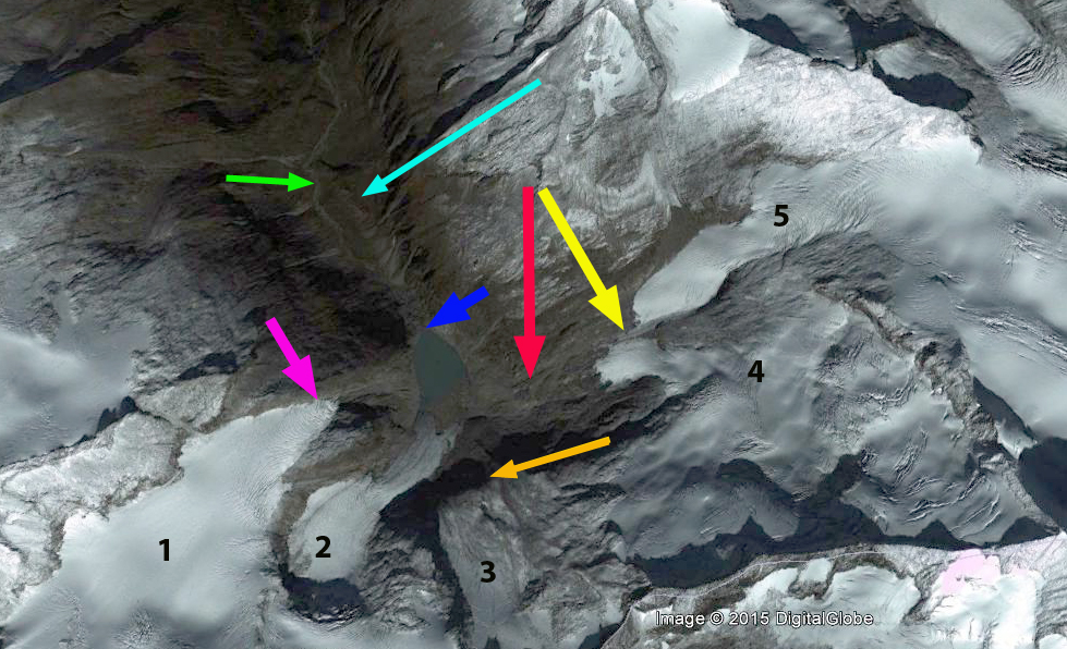
Yes, given that the Austrian Glacier Inventory has reclassified the glacier as five separate glaciers (Fischer et al, 2014). In this post they are numbered 1=Krimmlertorl Kees, 2=Obersulzbach Kees, 3=Bleidacher Kees, 4=Sulzbacher Kees, 5=Venediger Kees.
Nick Fisher sent me a map of the glacier prepared by the Austrian Military in the early 1930’s this is compared to the GE image of the glacier from 2012, below. According to this map, in 1934 the ice was at least 150 m deep over the current lake surface, where all the glacier streams united before heading down the ice fall. In 1934 the five branches of the Obersulzbach all joined and continued downglacier past a prominent rib on the east side of the glacier, light blue arrow, to terminate at 1980 meters, green arrow. The two western most glaciers Krimmerlertorl and Obersulzbach on the images, were joined at the pink arrow in 1934 and are well separated in 2012. At the orange arrow in 1934 Bleidacher (3) flowed over a steep cliff and joined the other segments. Today the glacier section ends at the top of a steep cliff. Glacier Sulzbacher and Venediger are the largest and easternmost draining the actual slopes of Großvenediger. They joined the other segments in 1934. By 1988 they had retreated to the red arrow but the two were still joined, by 2012 they had separated at the yellow arrow. Hence, we now have separate glaciers that formerly joined together. The World Glacier Monitoring Service reports indicate this glacier retreated 140 meters from 1991-2000 and 345 m from 2001-2010, a substantial increase. Here we examine Landsat imagery from 1988, 1998, 2012, 2013 and 2014 to identify the retreat andand separation of the glacier into. By 1998 a small lake less than 100 m long has formed at the end of the glacier, blue arrow.
Map of the Obersulzbach Region in 1934 from Nick Fisher
Google Earth image from 2012
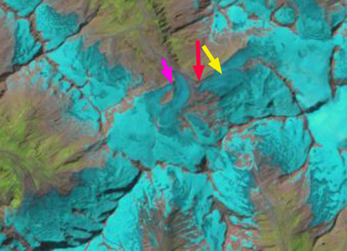
In 1988 there is no lake visible at the end of the main terminus. The glacier has retreated 1.4 km since 1934. At the pink arrow glacier Krimmerlertorl and Obersulzbach are still joined in 1988. Glacier Sulzbacher and Venediger are also still joined at the yellow arrow and terminate at the red arrow. Glacier section Bleidacher has become detached.
By 1998 Krimmerlertorl and Obersulzbach are separated but the eastern glaciers Sulzbacher and Venediger are still joined at the yellow arrow. No lake yet exists at the terminus. Obersulzbach Glacier receded in a narrow bedrock basin since the late 1990’s and a shallow lake, Obersulzbach-Gletschersee, has formed since 1998 (Geilhausen et al, 2012). They observed that in 2009, the lake had an area of 95,000 m2 with a maximum depth of 42 m.
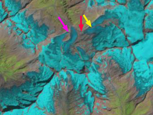
By 2013 all the glacier segments are separate. By 2013 the lake, Obersulzbach-Gletschersee,has grown to a length of 450 m and a with of over 200 meters. The retreat from 1988-2013 of glaciers Krimmerlertorl=0.8 km, Obersulzbach=0.6 km, Bleidacher=1.3 km, Sulzbacher=1.4 km, Venediger=1.6 km. The 2014 image is not as clear, but further retreat did occur. The Austrian Alpine Club 124th annual survey indicated 86% of Austrian glaciers retreated from 2013-2014.
The Salzach is fed by many glaciers covering over 100 square kilometers (Koboltschnig and Schoner, 2011). These glaciers melt all summer providing considerable runoff to the numerous hydropower projects along the Salzach, that can produce 260 MW of power. The Verbund Power Plant producing 13 MW is seen below, at blue arrow. Glacier area loss will lead to declines in summer runoff. A mass balance program has been started on Venediger Kees.
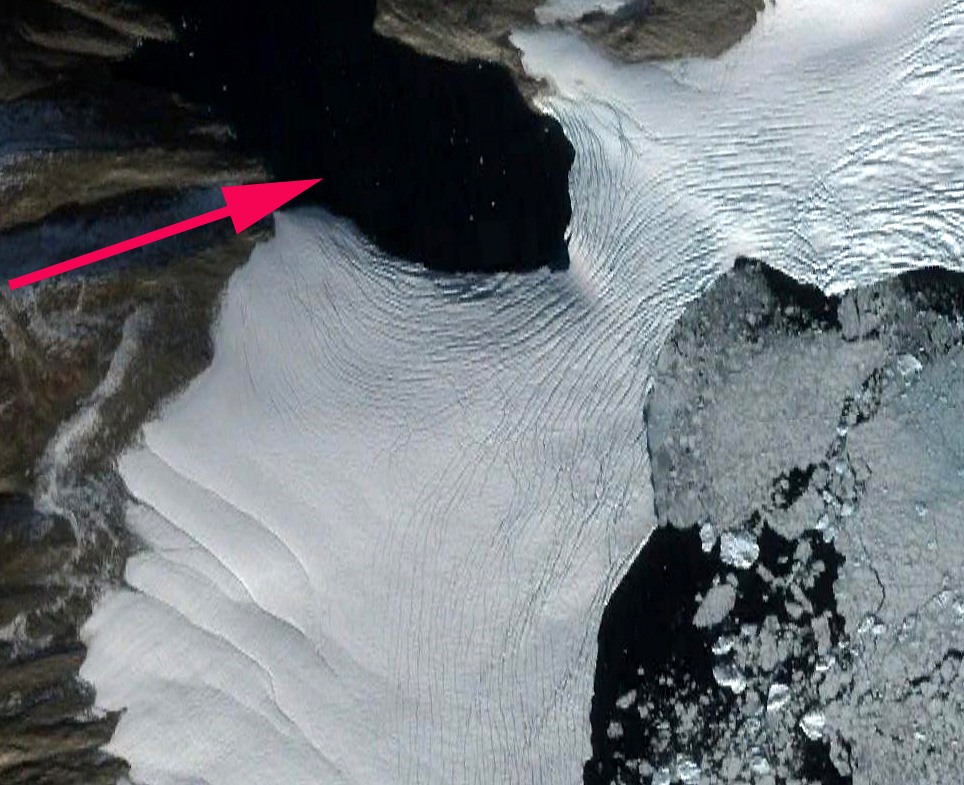
The retreat of outlet glaciers along the Greenland coast continues to change the maps of the region, Steenstrup Glacier located at 75.2 N in Northwest Greenland is an example of this. The glacier terminates on a series of headlands and islands, the glacier immediately to the south is Kjer Glacier. The boundary between Steenstrup Glacier and Kjer Glacier is Red Head, Steenstrup Glacier’s northern margin is near Cape Seddon. Here we examine changes in the terminus position of Steenstrup and Kjer Glacier from 1999 to 2014. The retreat of the glacier during this interval has led to generation of new islands. Steenstrup Glacier has retreated 10 km over the past 60 years (Van As, 2010). A recent example of the retreat is the separation from the glacier of an island in 2014. In 2012 there was a narrow glacier connection, red arrow, with an island Tugtuligssup Sarqardlerssuua that is clearly not stable, based on narrowness and extensive crevassing, the connection remained in 2013 and was in 2014.
Google Earth 2012 image Cape Seddon/Tugtuligssup Sarqardlerssuua, how long will this connection last? Less than two years.
Landsat image comparison of 2013 and 2014 of Cape Seddon/Tugtuligssup Sarqardlerssuua separation from Steenstrup Glacier.
Image from Van As (2010).
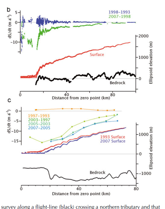
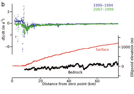
McFadden et al (2011) noted several glaciers in Northwest Greenland; Sverdrups, Steenstrup, Upernavik, and Umiamako that had similar rapid thinning patterns of up to ~100 m a-1 since 2000. They further noted that thinning was not synchronous with Steenstrup and Sverdrups thinning fast from 2002 to 2005, Upernavik from 2005 to 2006, and Umiamako from 2007 to 2008. This is not exactly synchronous, but occurring within a few years is essentially synchronous in terms of glacier dynamics. Each glacier also had a coincident speed-up with a 20% acceleration for Steenstrup Glacier (McFadden et al, 2011). Kjer Glacier was noted as relatively stable until loss of connection with Red Head Peninsula in 2005 (Van As, 2010). This is a familiar pattern with thinning there is less friction at the calving front from the fjord walls and the fjord base, leading to greater velcoity. The enhanced flow leads to retreat and further thinning, resulting in the thinning and the acceleration spreading inland. The initial thinning comes from a combination of basal and surface melt. This has been the primary mechanism for increased velocity of outlet glacier of the Greenland Ice Sheet.
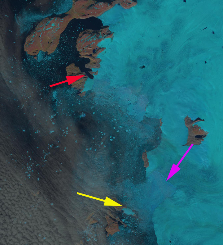
Here we examine Landsat images from 1999, 2013 and 2014 to identify changes of Steenstrup and Kjer Glacier. The yellow arrow indicates Red Head, which the glacier still reaches in 1999, though the connection is less than 2 km wide. The purple arrow indicates the ice front just north of Red Head that extends nearly due north to the next island at the icefront. The red arrow indicates the ice front of Steenstrup Glacier at Tugtuligssup Sarqardlerssuua. By 2013 the connection to Red Head has been lost, it is now an island, this occurred as noted by Van As (2010) in 2005. Retreat from Red Head is 6 km by 2013. There is a substantial embayment that develops, purple arrow southwest of an island still embedded in the icefront, indicating 4 km of retreat. North of this island that will soon lose it connection to the ice sheet, the embayment has expanded as well. The connection to the island at the north end of Kjer Glacier, has become much narrower since 1999 and will follow the route of Red Head and Tugtuligssup Sarqardlerssuua. In 2014 Steenstrup Glacier at the red arrow has separated from Tugtuligssup Sarqardlerssuua. The island west of the purple arrow still acts as a pinning point having stabilized the ice front here since 1975, but is now isolated in the same way as Red Head in 1999 and will soon be released from the glacier. From 2013 to 2014 the embayment is spreading inland and north.
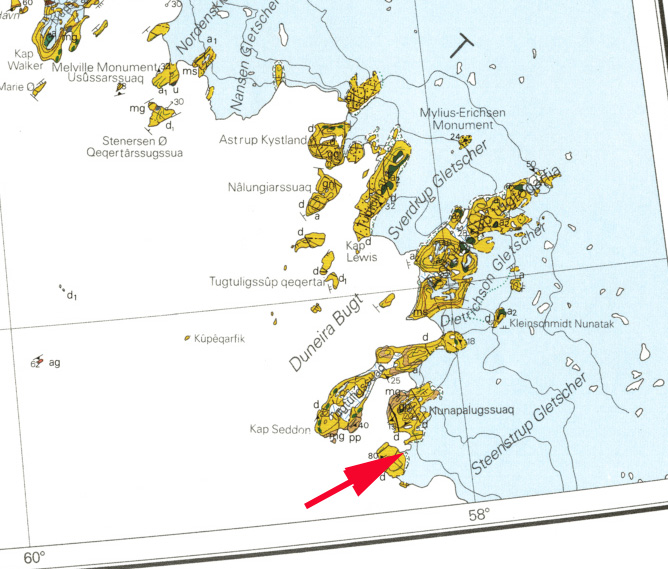
The retreat here is coincident with the thinning and acceleration and follows the pattern of retreat and new island generation seen at Kong Oscar Glacier, Alison Glacier and Upernavik Glacier. The map of Greenland is continues to change at an accelerated rate, bottom image is a geologic Map from the Geological Survey of Denmark and Greenland. Red arrow again indicates Tugtuligssup Sarqardlerssuua.
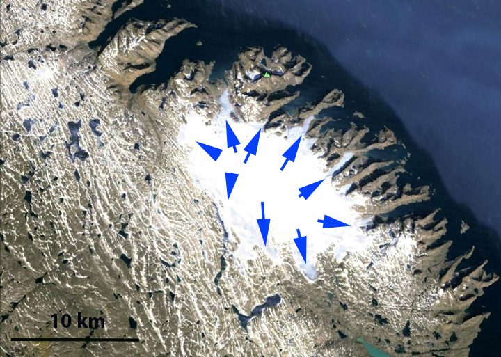
The Grinnell Ice Cap Is located on the Terra Incognita Peninsula on Baffin Island. The name suggests the reality that this is a not often visited or studied region. Two recent studies have changed our level of knowledge. Way (2015) notes that the ice cap has lost 18% of its area from 1974 to 2013 and that the rate of loss has greatly accelarated and is due to summer warming, declining from 134 km2 in 1973-1975 imagery to 110 square kilometers in 2010-2013 images. Papasodoro et al (2015) report the area in 2014 at 107 km2 with a maximum of elevation of close to 800 m. The location on a peninsula on the southern part of the island leads to higher precipitation and cool summer temperatures allowing fairly low elevation ice caps to have formed and persisted. Way (2015) in the figure below indicates the cool summer temperatures have warmed more than 1 C after 1990. Recent satellite imagery of snowcover and ICESat elevation mapping suggest little snow is being retained on the Grinnell Ice Cap since 2004. Papasodoro et al (2015) identify a longer mass loss rate of -0.37 meters per year from 1952-2014, not exceptionally different from many alpine glaciers. They further observed that from 2004-2014 this rate has accelerated to over -1 meter per year, including a thinning rate above 1.5 meters along the crest of ice cap. This can only be generated by net melting not ice dynamics. Further such rapid losses will prevent retaining even superimposed ice. Here we examine Landsat imagery from 1994 to 2014 to illustrate glacier response.
Grinnell Ice Cap in Google Earth
From Way (2015)
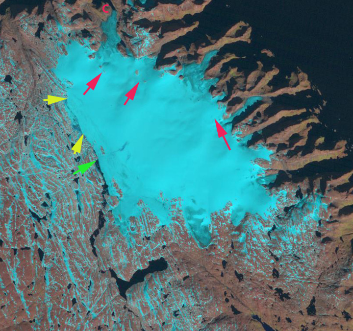
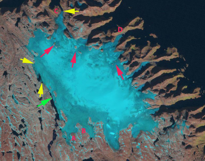
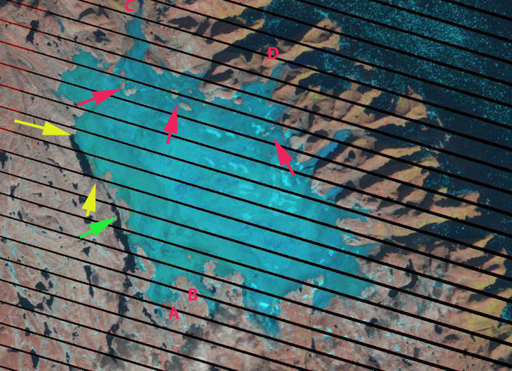
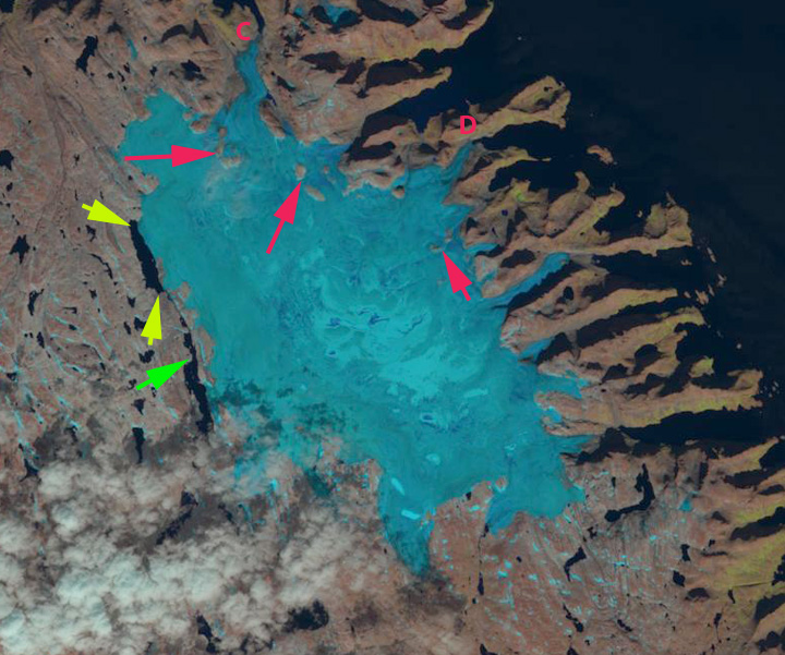
The red arrows in each image indicate areas of small nunataks that have begun to expand in the last decade. The yellow and green arrows indicate specific locations on the western margin of the ice cap where lakes are developing. Point A-D note specific locations adjacent to ice cap outlet glaciers. In 1994 the late August image indicates snowcover across most of the ice cap. The green arrow is at the northern end of a narrow lake. The yellows arrows are at the northern and southern end of a narrow ice filled depression. The nunatak area exposed at the red arrows is limited. At Point C the terminus is tidewater. In 2000 snow pack covers 40% of the ice cap. A small lake is developing at the yellow arrows. The glacier reaches the ocean at Point C and D. The glacier extends south of Point A and the outlet glacier at Point B is over a 1.2 km wide. In 2012 a warm summer led to the loss of all but snowpack on the glacier. At the red arrows the nunataks have doubled in size. At the yellow arrows a 2.5 km long lake has developed. At the green arrow a lake that has developed, is now separated from the glacier margin by bedrock. The glacier now terminates north of Point A. In 2014 again snowcover is minimal with two weeks left in the melt season. The outlet glaciers at Point C and D are no longer significantly tidewater. At Point B the outlet glacier is less than 0.5 km wide. The lake at the yellow arrows is 3 km long and 400 m wide. Some nunataks are coalescing with each other or the ice cap margin. The majority of the western margin of the ice cap has retreated 300-500 m. This retreat is surpassed at outlet glaciers by Point A and C. What is of greatest concern is the loss in thickness of over 1.5 per year on the highest portions of the ice cap, indicating no consistent accumulation zone. This results from the persistent loss of nearly all snowcover in the summer. This pattern of limited end of summer retained snowcover seen in most years since 2004, is a snow deficit that this ice cap cannot survive in our current warmer climate (Pelto, 2010). Way (2015) projects that that if the observed ice decline continues to AD 2100, the total area covered by ice at present will be reduced by more than 57%. Given the recent increases and lack of retained snowcover, suggests an even faster rate is likely.
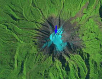
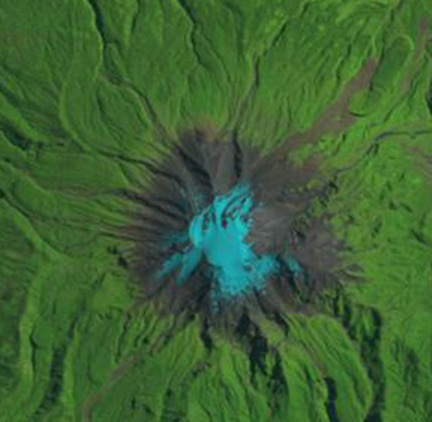
Calbuco Volcano in Chile erupted this week. It has been noted that significant pyroclastic flows/lahars have been observed travelling down the Rio Blanco fed in part by glacier melt. Here we examine the glaciers on Calbuco. We start with a 2012 Google Earth image that provides the clearest view. There are three primary glaciers, the main summit ice cap , a glacier below the western rim, that is not significantly connected to the main ice cap in 2012 and a glacier descending the southwest flank. There are numerous wind sculpted features observed from north-northeast to south-south west that also align with the flank glacier, blue arrows.
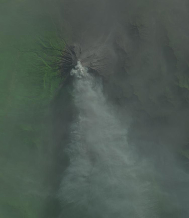
The extent of retained snowcover in 2012 is quite poor, purple dots which would lead to significant mass balance loss and thinning. There are two locations of expanding bedrock exposure with glacier thinning, red arrows. A review of available satellite imagery indicates that most years the summit ice cap retains good snow pack, but not in recent years with 2012, 2014 and 2015 having limited snowpack. The 2015 image is from March 26th just four weeks before the eruption. As in 2012 the glacier had lost almost all of its snowpack and was experiencing a large volume loss in 2015. This post will be updated with post eruption Landsat imagery when clear view is available. The last image in the post is from 4/27/2015 with the eruption ongoing, whether the glacier is completely gone or buried in ash impossible to discern.
2012 Google Earth image of Calbuco Volcano glaciers.
An examination of satellite imagery from 1985, 1998 and 2000 indicate this. Since the majority of the glacier is right at the summit the eruption will lead to the loss of this glacier. Given the size of the main summit ice cap glacier, area of 0.95-1.05 square kilometers, a range of volume scaling method provides a volume estimate of 0.02 cubic kilometers of ice (Grinsted, 2013). The volume of glaciers has likely been limited by the frequency of eruptions in the last two centuries,; however, the volume has not been sustainable with current climate. The two main rivers draining the southwest flank glacier and summit ice cap drain south to Lago Chapo, yellow arrows. The volume of water is limited and since it is early fall snowpack on the mountain was limited as well. The lahars from glacier melt cannot match those frequently seen in Iceland such as with Eyjafjallajökull.
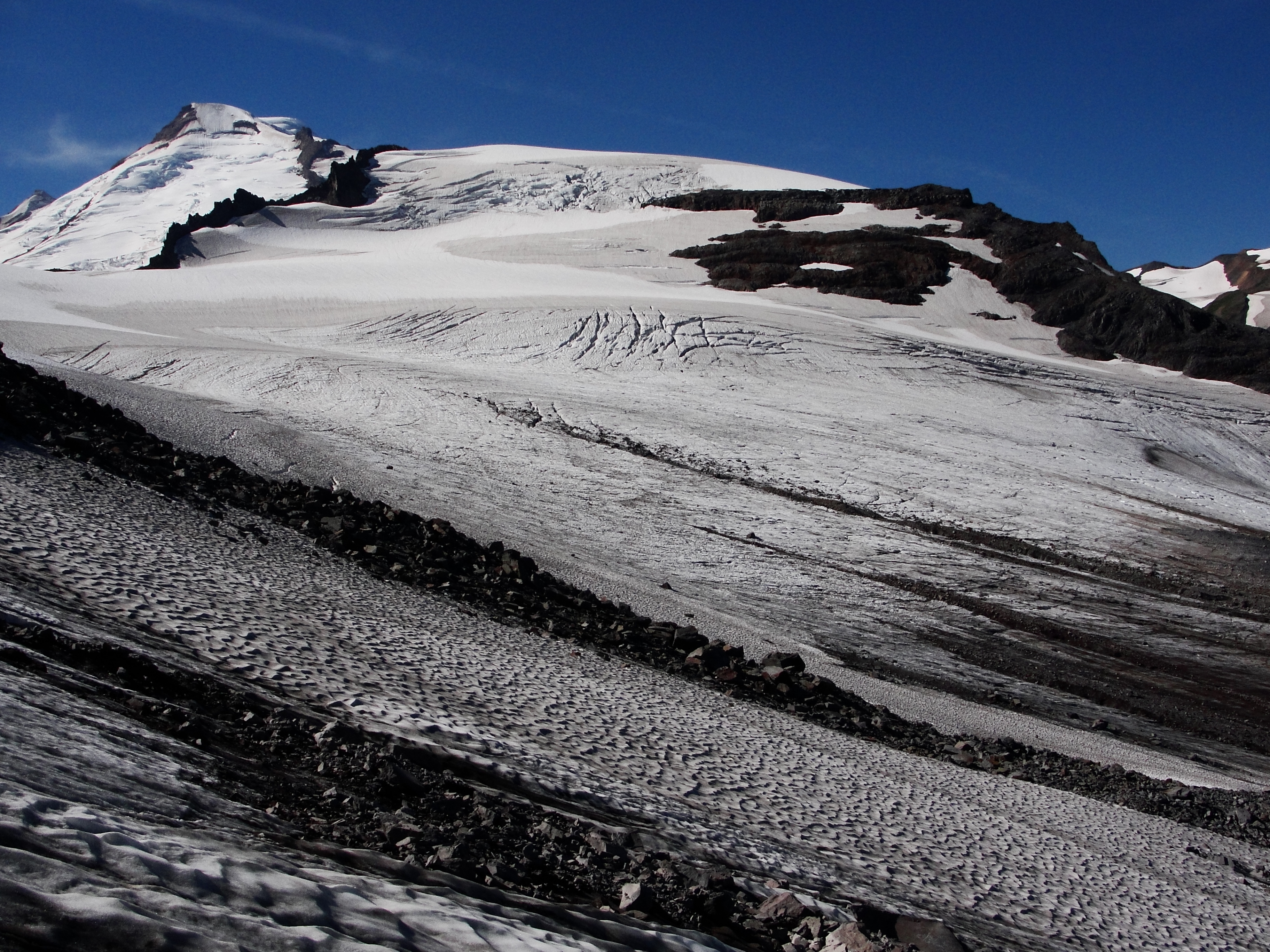
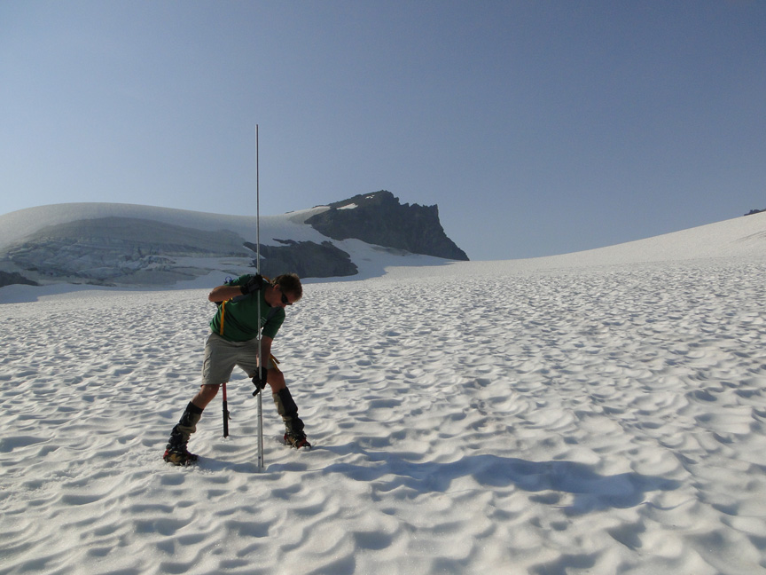
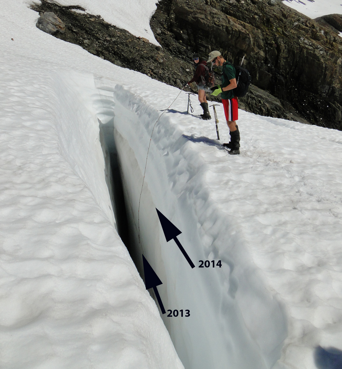
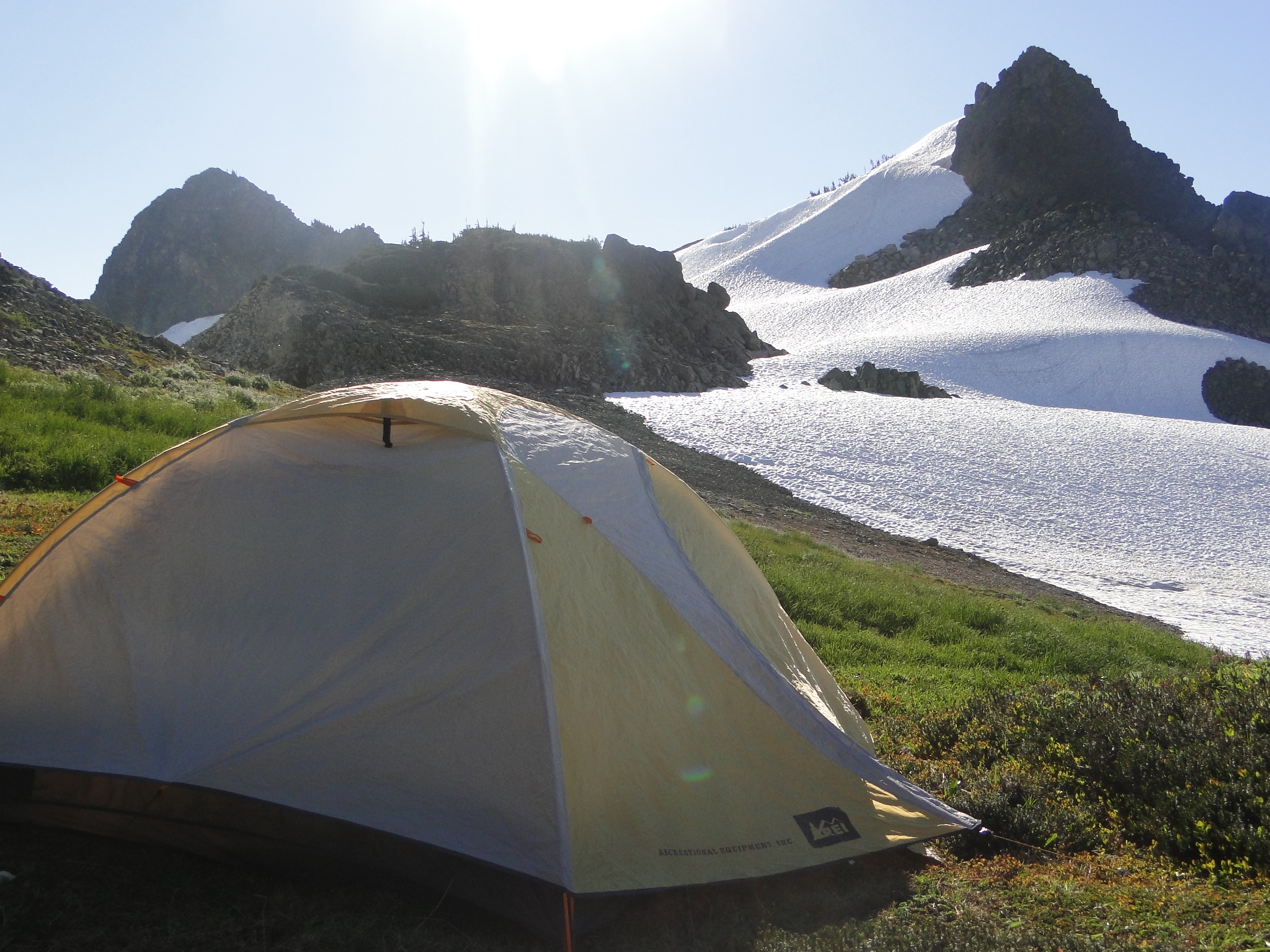
Annual mass balance is the difference between ice and snow added to the glacier via accumulation and snow and ice lost via ablation and in some cases calving. Alpine glacier mass balance is the most accurate indicator of glacier response to climate and along with the worldwide retreat of alpine glaciers is one of the clearest signals of ongoing climate change (WGMS,2010). For 25 consecutive years we (North Cascade Glacier Climate Project) have measured the mass balance of Sholes Glacier. On Sholes Glacier in 2014 we completed 162 measurements of snowpack depth using probing and crevasse stratigraphy, mainly probing on this relatively crevasse free glacier. We mapped the extent of snowcover on several occasions, and using the retreat of the snowline and stakes emplaced in the glacier observed the rate of ablation (melting). We also measured runoff from the glacier in a partnership with the Nooksack Indian Tribe, which provided an independent measure of ablation. The final mass balance in 2014 was -1.65 m of water equivalent, the same as a 1.8 meter thick slice of the glacier lost in one year. In 2014 we arrived at Sholes Glacier to find it already had 15% blue ice exposed, on August 7th. This had expanded to 25% by August 12th. This rapidly expanded to 50% by August 23rd, note Landsat comparison below. The snow free area expanded to 60% by the end of August and then close to 80% loss by the end of the summer. Glaciers in this area need 60% snowcover at the end of the melt season to balance their frozen checkbook. This percentage is the accumulation area ratio. This mass balance data is then reported to the World Glacier Monitoring Service, along with about 110 other glaciers around the world. Unfortunately the WGMS record indicates that Global alpine glacier mass balance was negative in 2014 for the 31st consecutive year. The video below explains how we measure mass balance each year with footage from the 2014 field season. Of course a key aspect is hiking to the glacier and camping in a tent each year.
The Sholes Glacier thickness has not been measured, but there is a good relationship between area and thickness, that suggests the glacier would average between 40 and 60 m in thickness. The 15 m of water equivalent lost from 1990-2014 is equal to nearly 17 m of ice thickness, which would be at least 35% of the glaciers volume lost during our period of measurement.
Sholes Glacier on August 7, 2014 and Sept. 15 2014, the glacier had lost 80% of its snowcover at this point an indicator of poor mass balance 2014.
Landsat 8 images of Sholes Glacier in 2014, with red line indicating snow line.
Measuring Accumulation on a glacier using Probing and crevasse stratigraphy.
Base Camp where we have spent more than 100 nights in a tent in the last three decades.
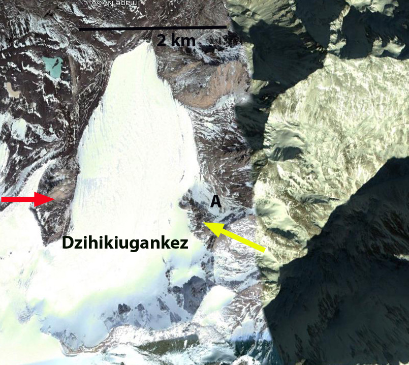
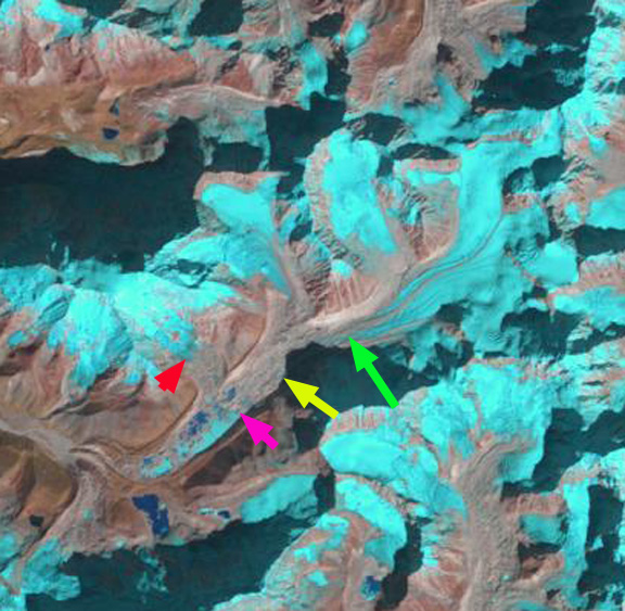
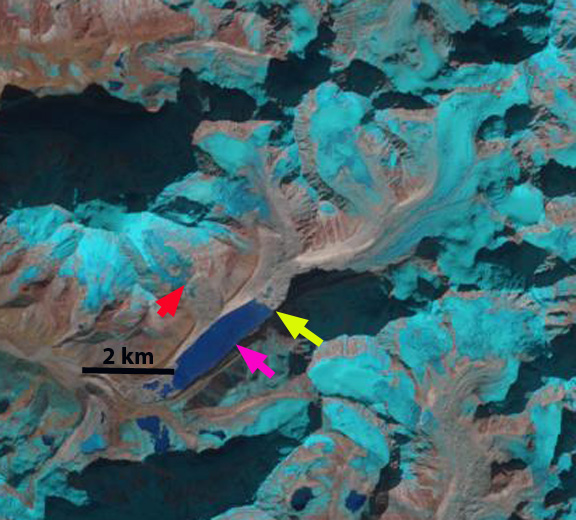
Dzhikiugankez Glacier (Frozen Lake) is a large glacier on the northeast side of Mount Elbrus, the highest mountain in the Caucasus Range. The primary portion of the glacier indicated in the map of the region does not extend to the upper mountain, the adjoining glacier extending to the submit is the Kynchyr Syrt Glacier. The glacier is 5 km long extending from 4000 m to 3200 m. Shahgedanova et al (2014) examined changes in Mount Elbrus glaciers from 1999-2012 and found a 5% area loss in this short period and accelerated retreat from the 1987-2000 period. As examination of Landsat images indicates Dzhikiugankez Glacier has the lowest percent of overall snowcover, as seen in the satellite image from August 2013 with the transient snow line shown in purple. The amount of blue ice is apparent on Dzhikiugankez Glacier (D). The main changes in this glacier are not at the terminus, but along the lateral margins, indicating substantial vertical and lateral thinning. Here we examine Landsat imagery from 1985 to 2013 to identify changes. In each image the red arrow indicates bedrock on the western margin, the yellow arrow bedrock on the eastern margin, Point A an area of glacier ice extending to the upper eastern margin, the purple arrow a medial moraine exposed by retreat and the green arrow the 1985 terminus of the glacier.
Map of northeastern side of Mount Elbrus, summit on left. Dzhikiugankez Glacier (Dzhikaugenkjoz) is outlined in black.
August 2013 Satellite image of Mount Elbrus
Google Earth image 2013
In 1985 the glacier connects beneath the subsidiary rock peak at the red arrow, a tongue of ice extends on the east side of the rock rib at the yellow arrow, Point A. The transient snow line is at 3550 m and less than 30% of the glacier is snowcovered. The medial moraine at the purple arrow is just beyond the glacier terminus. In 1999 the subsidiary peak is still surrounded by ice and the tongue of ice at Point A though smaller is still evident. The snowline is quite high extending to 3750 m, leaving only 10-15% of the glacier snowcovered. In 2001 the main terminus has retreated from the green arrow. A strip of rock extends up to the red arrow. The snowline is at 3500 m, with a month of melting left. In 2013 a wide zone of bare rock extends up to the subsidiary peak at the red arrow. The medial moraine, purple arrow is exposed all the way to its origin near the red arrow. In 2013 the tongue of ice at Point A, is gone. This glacier is retreating faster on its lateral margins as at the terminus, a 20% reduction between red and yellow arrows from 1985 to 2013. The snowline is at 3600 m, with several weeks of the melt season left. The key problem for the Dzhikiugankez Glacier is that there is an insufficient persistent accumulation zone. Pelto (2010) noted that a glacier cannot survive without a persistent and consistent accumulation zone, which Dzhikiugankez Glacier lacks despite being on the flanks of Mount Elbrus. Retreat of this glacier is similar to Azau Glacier, particularly the west slope of this glacier, and Irik Glacier. Unlike these glaciers it cannot survive current climate. The glacier is large and the glacier will not disappear quickly. Shahgedanova et al (2014) note the expansion of bare rock areas adjacent to glaciers on the south side of Mount Elbrus including Azau and Garabashi.
Menlung Glacier is one valley north of the China/Tibet border with Nepal and on the south side of Menlungste Peak. Menlung Glacier has a glacier lake at its terminus that is dammed by the glacier’s moraine. The glacier began to withdraw from the moraine and the lake began to develop after the 1951 expedition to the area. The glacier lake is at 5050 meters, the glacier descends from 7000 meters with the snowline recently around 5500 meters. The lower section of the glacier is heavily debris covered, which when the debris is more than several centimeters thick as in most areas here, reduces the rate of glacier melt. Melt is highest around the supraglacial lakes (shallow lakes on glacier surface), which can lead to the lakes expanding and coalescing. Benn (2001) examined the process on nearby Ngozumpa Glacier, Nepal. This region has experienced significant mass loss of -0.25 m/year from 2000-2010 (Gardelle et al, 2013). The Japanese Aerospace Exploration Agency has a side by side 1996 and 2007 satellite imagery that indicates the Menlung Glacier Lake developing in 1996 that still has remnant glacier ice in it, that is melted by 2007. Here we use Landsat imagery and Google Earth imagery to identify the changes from 1992-2014.
1992 Landsat image: In each image the pink arrow is the 1992 terminus, the yellow arrow the 2014 terminus, the green arrow the furthest downglacier extend of clean glacier ice and the red arrow the lower margin of a tributary glacier in 2014.
In Landsat imagery from 1992 the lake is still developing from a system of supraglacial lakes interspersed with debris covered stagnant glacier sections. In 1994 there is little change, other than some of the lakes are frozen. In 2001 a contiguous lake has formed that is 500 m long and 600 m wide, though the main glacier front has changed little. The lake rapidly expanded to a length of 1900 meters by 2009. The glacier retreat is 500 meters, the other 300 meters of lake expansion is a continued growth at the moraine end of the lake as ice cored moraine continues to melt. By 2013 the lake has extended to a length of 2250 m, due solely to further glacier retreat. In 2014 has experienced a further 50-100 m of retreat from 2013. The lake is now 2300 m long, and is turning a darker blue color as the amount of glacier flour in it diminishes. A comparison of the terminus and lake using Google Earth images from 2005 and 2014 indicate the rapid lake growth in the last decade. The lower portion of the glacier remains debris covered, and appears stagnant, but has significant supraglacial lakes only with 400 meters of the 2014 terminus, suggesting the period of rapid retreat is nearly over. The region above the terminus in 2014 is dissected by a significant surface glacier stream that extends 2.5 km upglacier to the beginning of the first sections of debris free ice. That the river stays on the surface so long indicates the lack of crevassing and the stagnant nature of the ice. From 1992 to 2014 the area of clean glacier ice has also migrated 1 km upglacier, green arrows. The red arrows indicate a smaller glacier that has retreated further from the lake and has developed some substantial bedrock areas amidst the lower glacier between 1992 and 2014. The retreat and lake expansion parallels that seen at Longbasba, Reqiang, Sepu Kangri and Ngozumpa Glacier.
1994 Landsat image
2001 Landsat image
2009 Landsat image
2013 Landsat image
2014 Landsat image
2005 and 2014 Google Earth image comparison 2014 Google Earth images. Black arrows indicate supraglacial stream.
For the last 31 years the first week of August has found me on the Columbia Glacier in the North Cascades of Washington. Annual pictures of the changing conditions from 1984 to 2014 are illustrated in the time lapse video below. This is the lowest elevation large glacier in the North Cascades. Columbia Glacier occupies a deep cirque above Blanca Lake and ranging in altitude from 1400 meters to 1700 meters. Kyes, Monte Cristo and Columbia Peak surround the glacier with summits 700 meters above the glacier. The glacier is the beneficiary of heavy orographic lifting over the surrounding peaks, and heavy avalanching off the same peaks. This winter has been the lowest year for snowpack in the North Cascades in the 32 years we have worked here. Below is a comparison from August 1, 2011 with Blanca Lake below the glacier still frozen and a beautiful scene on April 4, 2015 with the lake not frozen taken by Karen K. Wang. The winter in the region was unusually warm, but not as dry as in California; however, in the snowmelt and glacier fed river basins summer runoff will be low this year.
Blanca Lake Aug. 1, 2011 on left, and April 4, 2015 on right (Karen K. Wang, www.karenkwang.com)
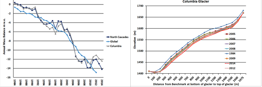
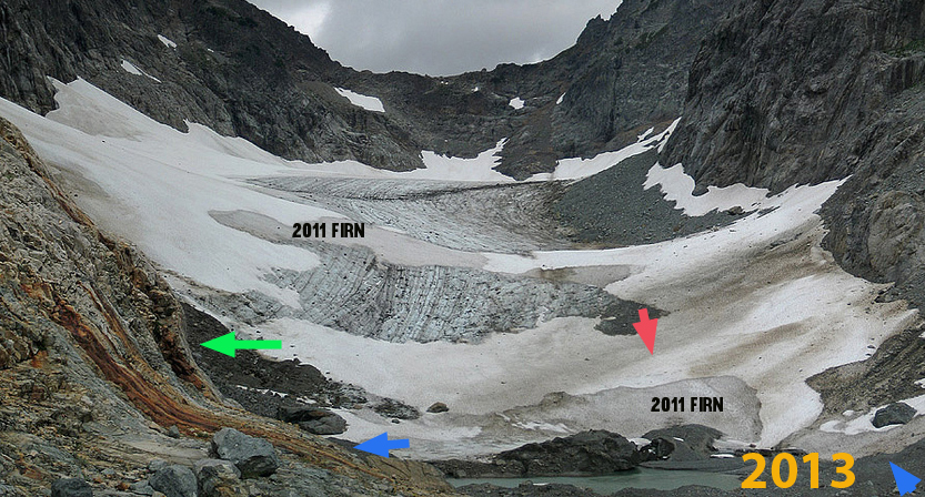
Over the last 31 years the annual mass balance measurements indicate the glacier has lost 14 meters of thickness. Given the average thickness of the glacier of close to 75 meters in 1984 this represents a 20% loss in glacier volume. During the same period the glacier has retreated 135 meters, 8% of its length. Most of the loss of volume of this glacier has been through thinning not retreat. To survive a glacier must have a persistent and consistent accumulation zone (Pelto, 2010). On Columbia Glacier in 1998, 2001, 2003, 2004, 2005, 2009 and 2013 limited snowpack was retained, resulting in thinning even on upper part of the glacier. This thinning of the upper glacier indicates the lack of a persistent accumulation zone such as in 2005, note the exposed annual ice and firn layers green arrows, this indicates the lack of retained accumulation in recent years. This indicates the glacier is in disequilibrium and cannot survive. Mapping of the glacier from the terminus to the head indicates a similar thinning along the entire length of the glacier. The overall mass balance loss parallels that of the globe and other North Cascade glaciers in the last three decades.
2005 Accumulation zone of Columbia Glacier
On left cumulative mass balance of Columbia Glacier compared to the WGMS global record and other North Cascade glaciers. On right change in surface elevation along the glacier from terminus to head indicating a 14-15 m thinning on average.
A comparison of images from 1986, 2007 and 2013 photograph provide a view of glacier change at the terminus. The blue arrows indicate moraines that the glacier was in contact with in 1986, and now are 100 meters from the glacier. The green arrow indicates the glacier active ice margin in 1986 and again that same location in 2007 now well off the glacier. The red arrow indicates the same location in terms of GPS measurements, this had been in the midst of the glacier near the top of the first main slope in 1986. In 2007 this location is at the edge of the glacier in a swale. The changes are more pronounced in 2013 as the terminus slope continues to decrease. The low snowpack in 2015 on the glacier in March, 2-3 m versus 6-8 m, will lead to considerable changes in the terminus this summer, that we will assess.
1986 Terminus Columbia Glacier
2007 Terminus Columbia Glacier
.
2013 Terminus Columbia Glacier
Jill Pelto painted the glacier as it was in 2009 (top) and then what the area would like without the glacier in the future, at least 50 years in the future (middle), and Jill at the sketching location (bottom), turned 180 degrees to view Blanca Lake. The lake is colored by the glacier flour from Columbia Glacier to the gorgeous shade of jade.
Clearly the area will still be beautiful and we will gain two new alpine lakes with the loss of the glacier. After making over 200 measurements in 2010 we completed a mass balance map of the glacier as we do each year. This summer we will be back again for the 32nd annual checkup. There will be likely be record low snowpack, comparable to 2005 the worst year from 1984-2014.
This is an index of posts on the response of specific Greenland glaciers to climate change. In the 1980’s when I first worked on Jakobshavn Isbrae, Greenland there was not much research occurring on the glaciers. Today in response to the dynamic changes discussed below and glacier by glacier in the index links, Greenland is the focus of numerous extensive, ongoing and important research projects. In 2015 scientists are gearing up for the main field season to better identify and understand the current and future response of this critical ice sheet. At the time of each post I reference the specific research relevant, the posts are from 2009-2014. In the intervening period new research has made some further advances, and I will endeavor to update each post to reflect this. The posts illustrate the significant response of Greenland Glaciers to climate change regardless of what type of glacier they are. The Polar Portal has developed an online viewer of change on selected glaciers. Each year the Arctic Report Card updates annual observations of Greenland Ice Sheet Change. The posts have benefitted from the insights and observations of Espen Olsen. Any questions about a glacier or suggestions on a glacier to look at let me know.
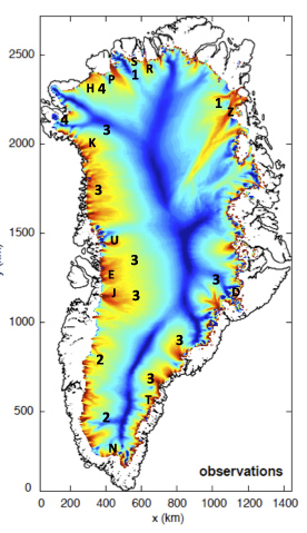
Base Map above right indicates the glacier types 1-4 distribution and key glacier locations with specific posts below. P=Petermann, R=Ryder, S=Steensby, H=Humboldt, Z=Zacharaiae, D=De Reste Bugt, T=Thyrm, N=Narssap Sermia, J=Jakobsan, E=Epiq Sermia, U=Umiamako, K=Kong Oscar.
Variations in Greenland Ice Sheet outlet glacier behavior
The Greenland Ice Sheet has an area of 2.17 million square kilometers (1.28 million square miles) and spans 18 degrees of latitude from north to south. It is not surprising that over this vast area that the geology and climate vary substantially and that this leads to variations in behavior of Greenland glaciers. Our tendency is to lump the Greenland Ice Sheet into one category impacted similarly by each of the dynamic forces that impact flow. This is akin to saying banks, credit unions and savings and loan institutions are impacted similarly by all the economic forces. In the case of a recession there is a shared signal, just as with global warming there is a shared signal among Greenland glaciers. This is a simplification that does not work. In this article we divide the glaciers into four main categories to illustrate the different properties and sensitiveness of each. This is an updated version of an article Dan Bailey and I wrote first for Skeptical Science, updated here with links above to the individual glaciers that emphasize the specific changes and with new references. In recent years the most striking aspect of Greenland Glaciers is that the signal of change is so strong and on so many of the different glaciers. The specific response is different, which if we try to lump the glaciers into one category, makes the data look noisy. Instead if we look at the response of glaciers with similar dynamics than the signal of response is strong indeed. Csatho et al (2014) note the variation in ice thickness across the ice sheet for the 1993-2012 period and that 48% of the thinning is driven by ice dynamics. The net loss is an equivalent contribution of 0.67 mm/year to sea level rise.
Greenland glaciers fall into at least 4 common types, each with its own unique sensitivity to sea surface temperature, surface melting, meltwater lubrication, calving changes, etc.
Type 1: Northern, with Large Floating Termini
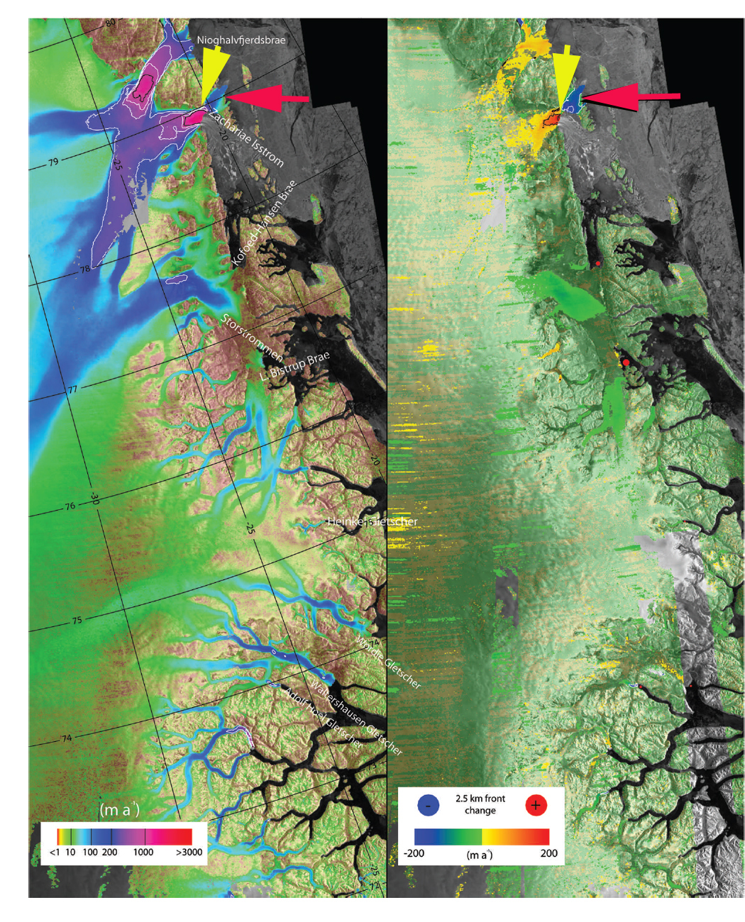
Northern glaciers with large floating termini (Petermann, Ryder, Steensby, Zachariae, Academy, etc). Each of these is a marine terminating outlet glacier that has an extensive floating ice shelf. The large ice shelves can exist in part due to the lower surface melt rates and the lower flow rates of the glacier. Petermann Glacier is the fastest with a flow speed of 1000 m/year at the grounding line. This is much less than the average outlet glacier speed along the west coast. The large floating ice shelves are susceptible to bottom melting but, except for Petermann Glacier, we have no observations of the process or that more warm water is penetrating under these ice shelves. Rignot and Steffen (2008) found that at Petermann Glacier 80% of the ice loss into the ocean was from basal melting of the floating tongue. If the ice shelves are removed, the feeding glacier is less buttressed and will accelerate for a period and draw down its surface profile. The recent ice area lost by Petermann, Steensby, Academy and Zachariae Ice Stream indicate these glaciers are being impacted by the increased melting at the surface and likely the base of the ice shelf for Petermann Glacier at least.
Examination of how far the high velocities extend inland in Figure 2 and 3 indicates that it is only Zachariae and Petermann that tap far into the ice sheet. This northern area has low accumulation rates, and a shorter less intense melt season. The early onset of melting and lack of accumulation in 2010 led to an early exposure of the ablation zone on these glaciers. This is their sensitivity Achilles Heel: relatively little increases in melt can expand the ablation zone appreciably given the low surface slopes and low accumulation rates. Based on the velocity map, it is the Zachariae that is likely the only of this group that would be comparable to a bank that is too big to fail as its increased velocity band extends well into the ice sheet (Joughin et al, 2010).
Figure 1. Velocity of Petermann and Humboldt Glacier, the latter does not have a deep bedrock trough extending to the heart of the GIS.
Fig 2. Ice flow speed for Zachariae Glacier (Joughin et al, 2010)
Type 2: Inland-terminating
Glaciers with inland termini lacking any calving (Sukkertoppen, Frederickshaab, Russell, etc). Between the fast flowing marine terminating outlet glaciers, the ice sheet particularly in the southwest quadrant has numerous glaciers that terminate on land or in small lakes. The velocity of these glaciers reaches a maximum of 1-2 meters/day. Each terminates on land because total ablation over the glacier equals total accumulation at the terminus. These glaciers are more like a typical alpine glacier and are susceptible to the forces that tend to cause alpine glaciers to experience peak flow during spring and early summer. Those forces are the delivery of meltwater to the base of the glacier, when a basal conduit system is poorly developed. This leads to high basal water pressure, which enhances sliding. As the conduit system develops the basal water pressure declines as does sliding, even with more water. In the long run it is not clear that more melt will lead to sustained higher velocities as a more efficient drainage system leads to lower basal water pressures. Sundal et al, (2011), best illustrated this.
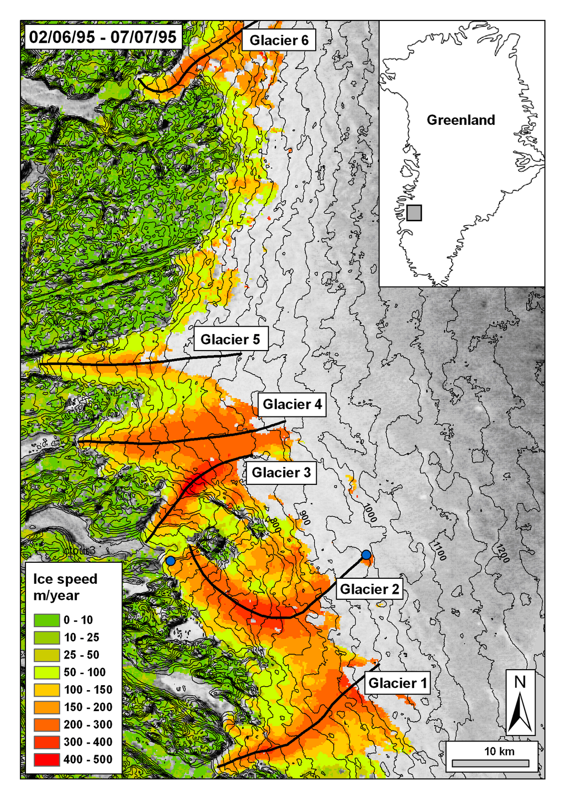
Fig 3. An example of a two-dimensional ice-velocity map of the study area in southwest Greenland Inland terminating glaciers velocities (Sundal et al, 2011).
This is what has been recently reported to be the case by Sundal et al (2011). The meltwater lubrication mechanism is real, but as observed is limited both in time and area impacted. It is likely that, as on alpine glaciers, the seasonal speedup is offset by a greater slowdown late in the melt season. Most observed acceleration due to high meltwater input has been on the order of several weeks, leading to a 10-20% flow increase for that period. The role of supraglacial lakes in this has been a point of emphasis; Luthje et al, (2006) noted that the area covered by supraglacial lakes was independent of the summer melt rate, but controlled by topography. This led Luthje et al (2006) to conclude that the area covered by supraglacial lakes will remain constant even in a warmer climate. This suggests that the enhancement of flow by the drainage of such lakes would be limited.
The land terminating glaciers such as Sukkertoppen, Russell and Mittivakkat are retreating significantly in response to global warming. This is an indication of negative mass balance. The latter glacier in southeast Greenland has retreated 1200 meters since 1931 (Mernild et al, 2011). The Mernild study identified this slow rate compared to the outlet glaciers and, based on mass balance observations, that the current surface mass balance can only support a glacier at most one-third its current size. This indicates the slow but inexorable sensitivity of the non-calving glacier to surface mass balance change. Moon and Joughin (2008) observed that the retreat of the land terminating glaciers was relatively minor from 1992-2007, averaging 5 m/year or less. These glaciers are the equivalent in our banking system to the local banks: there are many and they are sensitive, but the changes in a single one is not important.
Type 3: Marine-terminating
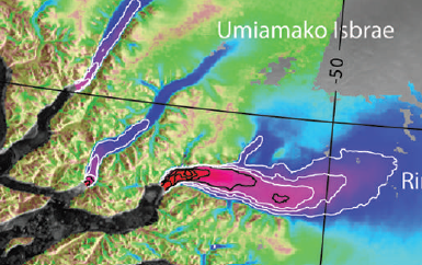
Fast flowing marine terminating outlet glaciers of western and southeast Greenland (Rinks, Umiamako, Helheim, Jakobshavn, Epiq Sermia, etc). These are the glaciers that drain the greatest area of the ice sheet and deliver the greatest volume to the oceans via calving. The flux from many of the larger glaciers is over 10 km3/year (DMI). Each of these glaciers is fast-flowing at the terminus; the fast flow section extends inland into the ice sheet up a sub-glacial trough. The outlet glaciers act like a drain capturing ice from a larger area of the ice sheet than their narrow terminus would suggest.
Figure 4. Umiamako Glacier is typical with the highest velocity near the calving front and the high velocity ice stream extending back into the ice sheet.
Figure 5. Jakobshavn Glacier terminus retreat, the recent retreat has been associated with thinning and faster flow.
Pelto et al (1989), a paper on the equilibrium state of the Jakobshavn Glacier, showed that the terminus had not changed significantly in 30 years; its velocity had also been consistent. Furthermore, it was observed that the velocity was consistent throughout the seasons. This indicated that the glacier velocity was not being impacted by the meltwater pulse each summer.
Bob Thomas (NASA, 2004) and Terry Hughes (University of Maine, 1986) developed the basic mechanism of flow for the glacier that has proven to be true. The outlet glaciers have a balance of forces at the calving front. The fjord walls, the fjord base and the water column impede flow. The slope of the glacier, its upglacier velocity and the height of the calving face strive to increase flow. If the glacier thins than there is less friction at the calving front from the fjord walls and the fjord base, leading to greater flow. The enhanced flow leads to retreat and further thinning, resulting in the thinning and the acceleration spreading inland. In 1990 it was not envisioned that acceleration would occur as soon as it has, yet that was the motivation for the research.
Fig 6. Jakobshavn profile (Thomas et al, 2009)
In 2001 acceleration of Helheim, Jakobshavn and Kangerdlussaq Glacier caught the attention of the world. By 2007, acceleration had been noted at all 34 marine terminating outlet glaciers observed.
The acceleration was not significantly seasonal; Howat et al (2010) noted a 15% seasonal component to the acceleration, it had spread inland and had led to retreat and thinning. This demonstrated that the marine terminating glaciers were largely responding to a change in the balance of forces at the glacier front.
Fig 7. Ice flow velocity as color over SAR amplitude imagery of Jakobshavn Isbræ in a) February 1992 b) October 2000. In addition to color, speed is contoured with thin black lines at 1000 m/yr intervals and with thin white lines at 200, 400, 600, and 800 m/yr. Note how the ice front has calved back several kilometers from 1992 to 2000. Further retreat in subsequent years caused the glaciers speed to increase to 12,600 m/yr near the front. (Ian Joughlin, Big Ice)
The recent increases in outlet glacier discharge have always been coincident with partially floating ice tongue losses. This causes reduced back pressure at the glacier front, letting up on the brakes; the resulting glacier thinning leads to less basal friction and further acceleration. If the glacier front retreats into deeper water the process will continue and increase. This is why understanding the basal slope changes inland of the calving fronts is crucial. Moon and Joughin (2008) observed the terminus change of 203 glaciers from 1992-2007 and noted a synchronous ice sheet wide retreat of tidewater outlet glaciers. The thinning could be due to increased surface melt, basal melt or most likely a combination of the two. Certainly the supraglacial lake drainages are not the key as the widespread acceleration in the southeast and southwest Greenland, yet the southeast has less than 10% of the lakes of the southwest , as documented by Selmes et al (2013) in a paper submitted to the Cryosphere.
Moon and Joughin (2008) reported for the 2000-2006 period:In the southeast quadrant 35 glaciers retreated an average of 174 m/year. In the eastern quadrant 21 glacier retreated an average of 106 m/year. In the northwest 64 glaciers retreated an average of 118 m/year. Each quadrant’s retreat increased markedly after 2000. In east central Greenland Walsh et al (2012) noted the retreat of all 37 outlet glaciers examined. Bjork et al (2012) note the terminus change in 134 east Greenland glaciers, idenitifying the last decade as the most rapid for marine terminating glaciers but not land terminating glaciers. The largest of this group are comparable to the banks that are too big for our banking system to allow them to fail: they drain a substantial portion of the entire ice sheet and reach so far into the ice sheet that their behavior can impact that of other adjacent glaciers.
Type 4: Marine-terminating in Shallow Water
Marine terminating glaciers outlet glaciers in shallower water (Humboldt, Cornell, Steenstrup etc). These glaciers do have calving termini, but lack the large fast flowing feeder tongues extending into the glacier. This is because there is not a topographic low under the ice sheet that funnels the flow. Humboldt Glacier is the widest front of any Greenland Glacier, wider even than Petermann Glacier. However, the velocity on average is low at 100 m/year and the base of the glacier is quite high. This makes it difficult for a large calving retreat of the glacier to occur and extend inland. Humboldt Glacier is retreating but as the velocity profile indicates the glacier, despite its size, does not tap dynamically into the center of the ice sheet. These glaciers are substantial, but their failure (though significant for sea level) would not destabilize the ice sheet as a whole. Naarsap Sermia would be another example in southwest Greenland. Dodge and Storm Glacier an example in northwest Greenland.
The amazing aspect of Greenland glaciers is that (despite the specific variation in type, location specific fjord configuration, etc) their response has been as uniform and synchronous to global warming as has been observed. If this warming of the world persists long enough, the ice “banks” of Greenland will begin to fail. Those with the greatest reserves on their asset sheets and the fastest turnover, and thus having the greatest potential contributions to sea level rise over time, are: In the north, Zachariae (and to a lesser extent, Petermann). The fast flowing marine terminating outlet glaciers of western and southeast Greenland (Rinks, Umiamako, Helheim, Jakobshavn, Epiq Sermia and Kangerdlussaq).
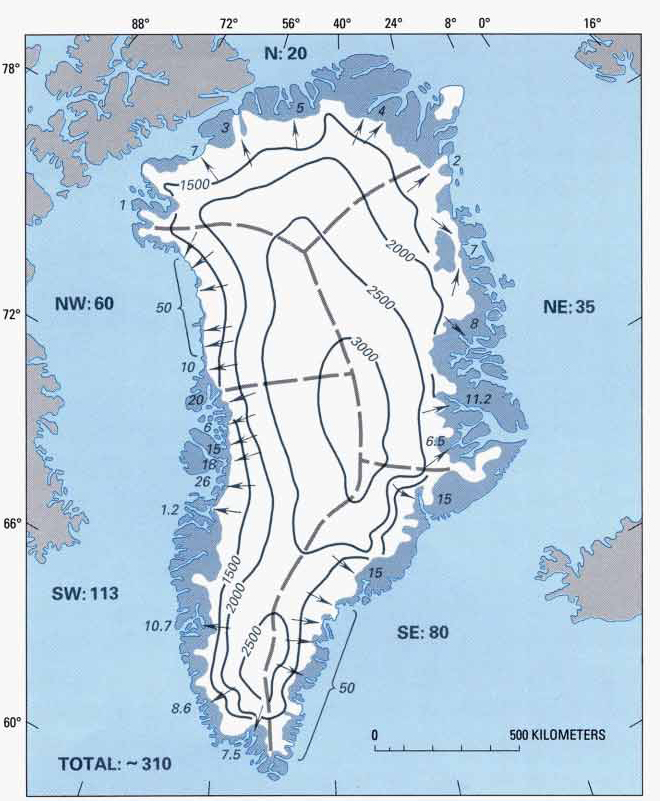
The surface mass balance of the glacier is the difference of accumulating snow on the ice sheet (its income) and snow and ice losses from melting and calving (its expenditures). The volume of the ice sheet is its asset. On an ice sheet, the main factor driving flow is simply the mass balance input in the accumulation zone. The higher the accumulation rate the faster the movement; the accumulated snow is inexorably moved downslope towards the ocean and the margin of the ice sheet. Observation of a precipitation map (focused not on the outer margin, but on the accumulation zone of the ice sheet) indicates that highest accumulation rates, over 40 cm per year, extend along the western side of the ice sheet to the southeast quadrant of the ice sheet. The southeast quadrant also has many fewer surface lakes than the southwest quadrant.
Figure 9. Mass balance in Greenland from Van Den Broecke et al, (2009)D denotes change in ice discharge while SMB denotes the net surface mass balance (accumulation minus ablation).)
Fig 10. Distribution of precipitation in Greenland (in grams per square centimeter per year). Contours dashed where inferred. Ice-free areas are shown in dark gray. (USGS, Satellite Image Atlas of Greenland)
The overall topography of the ice sheet is controlled both by the basal and peripheral geology and the mass balance distribution of the ice sheet. The higher rates of mass accumulation inland and the greater melting nearer the margin yield a steeper profile for the ice sheet.
Figure 11 shows that the contours have the closest spacing along the west margin and in the southeast, just as the high accumulation rates in those areas would suggest. Thus the combination of the surface slope and the accumulation rate drive faster flow in these regions.
Climate change has led to an observed increase in surface melting, surface accumulation, increased discharge and overall mass balance losses. The very mechanism that establishes the basics of behavior of the GIS mass balance are changing (Zwally et al, 2011). This is leading to most Greenland glaciers retreating, most outlet glaciers accelerating, an increase in the number and elevation of Greenland lake, expanding melt extent on the ice sheet. The 2012 seasons extraordinary ice melt extent is illustrated by the video below of Marco Tedesco’s melt extent data set. .
Leroux Bay is on the west coast of the Antarctic Peninsula in Graham Land. Numerous glacier drain from the Antarctic Peninsula into the ocean along this coast, and as they retreat the coastline is changing. Air temperatures rose by 2.5°C in the northern Antarctic Peninsula from 1950 to 2000, which has led to recession of 87% glaciers and ice shelves on the Peninsula in the last two decades (Davies et al.,2012). Most spectacularly has been the collapse of Jones, Larsen A, Larsen B, Prince Gustav and Wordie Ice Shelves since 1995 (Cook and Vaughan, 2010). This has opened up our ability to examine sediments that had accumulated beneath the floating ice shelves. The LARISSSA Project has been pursuing this option and utilized the Korean icebreaker ARAON to explore and map the bathymetry of Leroux Bay. Last week Antarctica recorded its highest temperature at the Argentine Base Esperanza on March 24th, 2015 located near the northern tip of the Antarctic Peninsula reported a temperature of 17.5°C (63.5°F). Here we examine the changes from 1990 to 2015 of glacier on the north side of Leroux Bay.
Google Earth image indicating glacier flow directions, blue arrows, island yellow arrow and glacier terminus red arrow.
In 1990 and 1991 the Leroux Bay Glacier extended to the yellow arrow, which is an island connected by the glacier to the mainland and acts as a stabilizing point for the glacier. The ice front is marked with yellow dots in both cases. The terminus region of the glacier is floating, making this a small ice shelf, fed by three tributaries, one from the north, one from the east and one from the northeast. By 2001 the glacier front has retreated to the red arrow, losing most of the floating area, and the northern tributary now has an independent calving front. The red arrow also points to the tip of a peninsula, another stabilizing point, the ice front is marked by the red dots for 2001 and 2015. The yellow arrow indicates the new island that is detached from the mainland. The two images from January 2015 and Late February 2015 indicate limited retreat an the north and south sides of the terminus, but retreat in the glacier center has led to a concave shaped calving front. Retreat from 1990 to 2015 averages 2.1 kilometers. The USGS map (Blue Line) indicates the terminus in the 1960’s was 3 km beyond the 1990 terminus location. The calving front remains active with extensive crevassing. It is not clear simply from Landsat imagery if any of the glacier is afloat, if so it would likely be the southern half of the eastern tributary, There is limited melting in this region, so volume loss can occur via basal melt via ocean water or calving. Even in a warm summer there is little visible evidence of surface melting in 2015. The widespread loss of mass from ice shelves in Antarctica is mainly via basal melting (Paolo et al, 2015). An examination of the coast in the region illustrates numerous other examples where glacier retreat has led to separation of islands, such as with the loss of the Jones Ice Shelf.
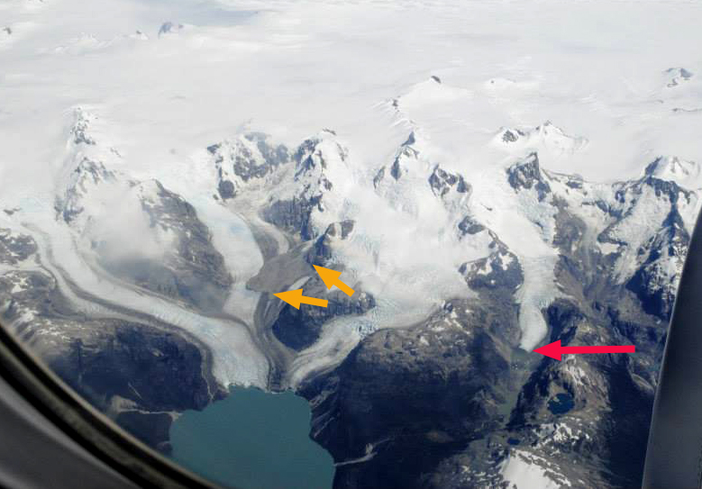
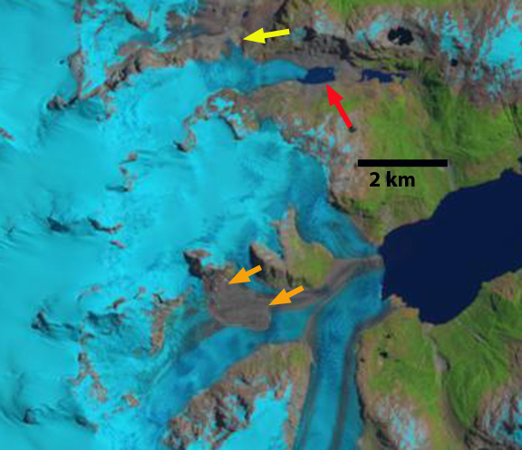
Jill Pelto, my daughter returning from fieldwork with UMaine in the Falkland Island took a picture last week out the plane window of Leones Glacier of the northern Patagonia Icefield. The picture illustrated two changes worth further examination, and the fact that if you have a glacier picture that you would like more information on let me know. The picture indicates outlet glaciers of the Northern Patagonia icefield fed by the snowcovered expanse. Also evident is a large landslide that is both fresh and that I knew had not been there before, orange arrow,and it showed a new lake had formed due to retreat of the glacier north of Leones Glacier, red arrow, hereafter designated North Leones Glacier. The landslide extends 2 km across the glacier and is 3 km from the terminus. Here we use 1985 to 2014 Landsat imagery to identify changes in North Leones Glacier and the landslide appearance.
Jill Pelto took this picture on March 13th, 2015
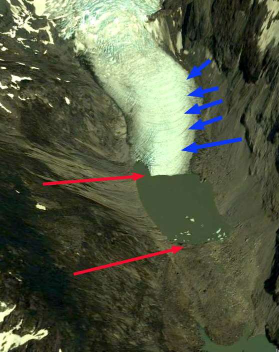
In 1985 there are medial moraines on the glacier surface, but no large landslide deposit. The Northern Leones Glacier terminates on land, red arrow. A distributary terminus almost connects with another glacier to the north at the yellow arrow. In 1987 there is little evident change from 1985. By 2002 a small lake is beginning to form at the terminus of Northern Leones Glacier. By Feb. 2014 a substantial lake has formed at the end of the North Leones Glacier. There is considerable separation between the distributary terminus at the yellow arrow and the next glacier. There is no landslide deposit either. Google Earth imagery indicates the lack of a landslide deposit as well. A closeup of the terminus of North Leones Glacier in 2013, with Google Earth imagery, indicates ogives (blue arrows), which are annually formed due to seasonal velocity changes through an icefall. In January 2015 the landslide deposit is evident, extending about 2 km across Leones Glacier and 3 km from the terminus. The North Leones Glacier has retreated 700 meters from 1985-2015. The retreat of the distributary terminus indicates thinning upglacier of the icefall on North Leones Glacier. The landslide adds mass to Leones Glacier, which will lead to a velocity increase. The debris is thick enough to reduce melting in this portion of the ablation zone. The velocity of this glacier is indicated by (Mouginot and Rignot, 2015) as 200-400 meters per year, indicating that for the next decade at least this landslide will impact the lower Leones Glacier. (Willis et al, 2012) identify thinning of the Leones Glacier area around 1 m per year, which will be reduced on the landslide arm of the glacier.
(Davies and Glasser, 2012), indicate that this region experienced increased area loss from 1986-2011. Lago Leones feeds the Leones River which is also fed by the retreating General Lago Carerra Glacier.


 Clearly the area will still be beautiful and we will gain two new alpine lakes with the loss of the glacier. After making over 200 measurements in 2010 we completed a mass balance map of the glacier as we do each year. This summer we will be back again for the 32nd annual checkup. There will be likely be record low snowpack, comparable to 2005 the worst year from 1984-2014.