Ampere-Lapparent Glacier Retreat, Kerguelen Island

ampere compare

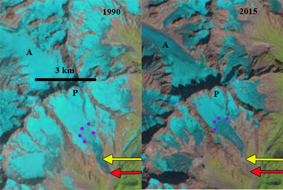
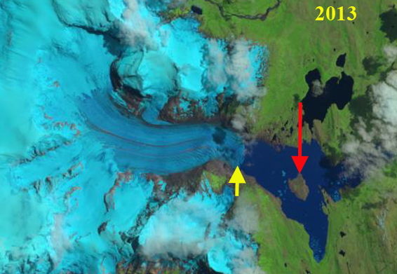
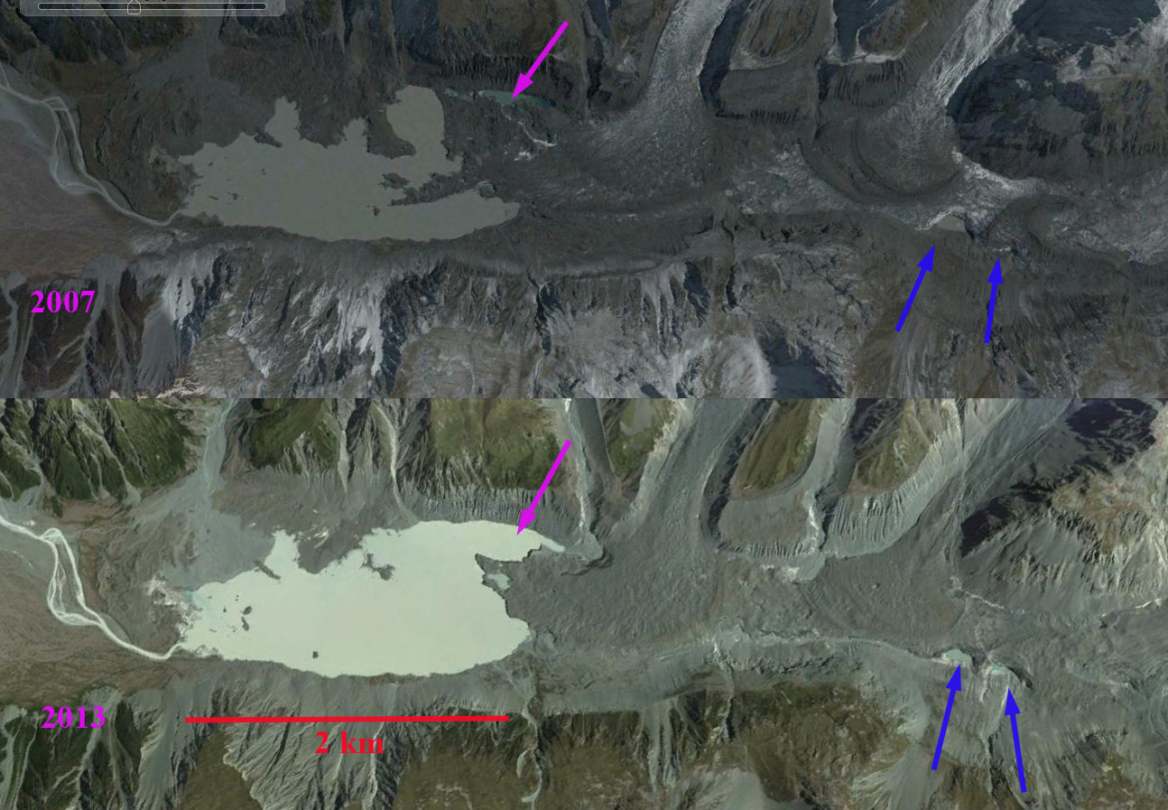
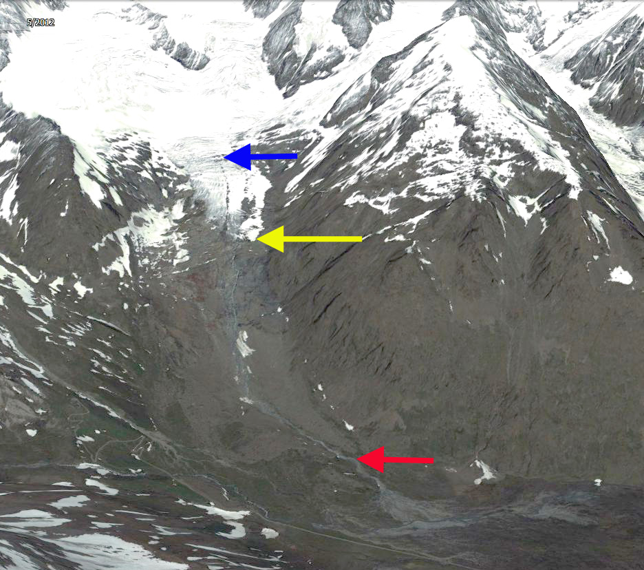
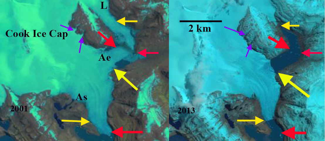
Comparison of Ampere Glacier (A) and Lapparent  Glacier (L) southern outlet glaciers of the Cook Ice Cap in 2001 and 2013 Landsat images; red arrow indicates 2001  terminus locations, yellow arrows 2013 terminus locations and purple arrow upstream thinning.

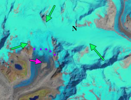
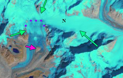
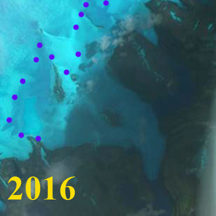
Kerguelen Island sits alone at the edge of the furious fifties in the southern Indian Ocean. The island features numerous glaciers, the largest being the Cook Ice Cap at 400 square kilometers. A comparison of aerial images from 1963 and 2001 by Berthier et al (2009) indicated the ice cap had lost 21 % of its area in the 38 year period.  Ampere Glacier is the most prominent outlet glacier of the Cook Ice Cap.  Berthier et al (2009) noted a retreat from 1963 and 2006 of 2800 meters of the main glacier termini in Ampere Lake (As). The lake did not exist in 1963. A second focus of their work was on the Lapparent Nunatak due north of the main terminus and close to the Ampere Glaciers east terminus (Ae). The nunatak expanded from 1963-2001, in the middle image below from Berthier et al (2009), but it was still surrounded by ice.  This is dominated by cloudy weather, with not a single good Landsat image of the glacier since 2013, the January 2016 indicates the snowline, purple dots is similar to 2001.

Kerguelen-Island-topo-Map

Map of Kerguelen Island

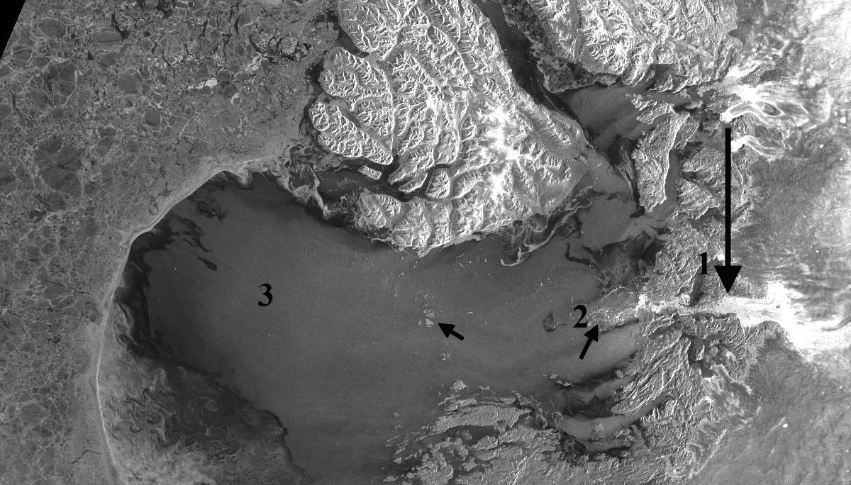
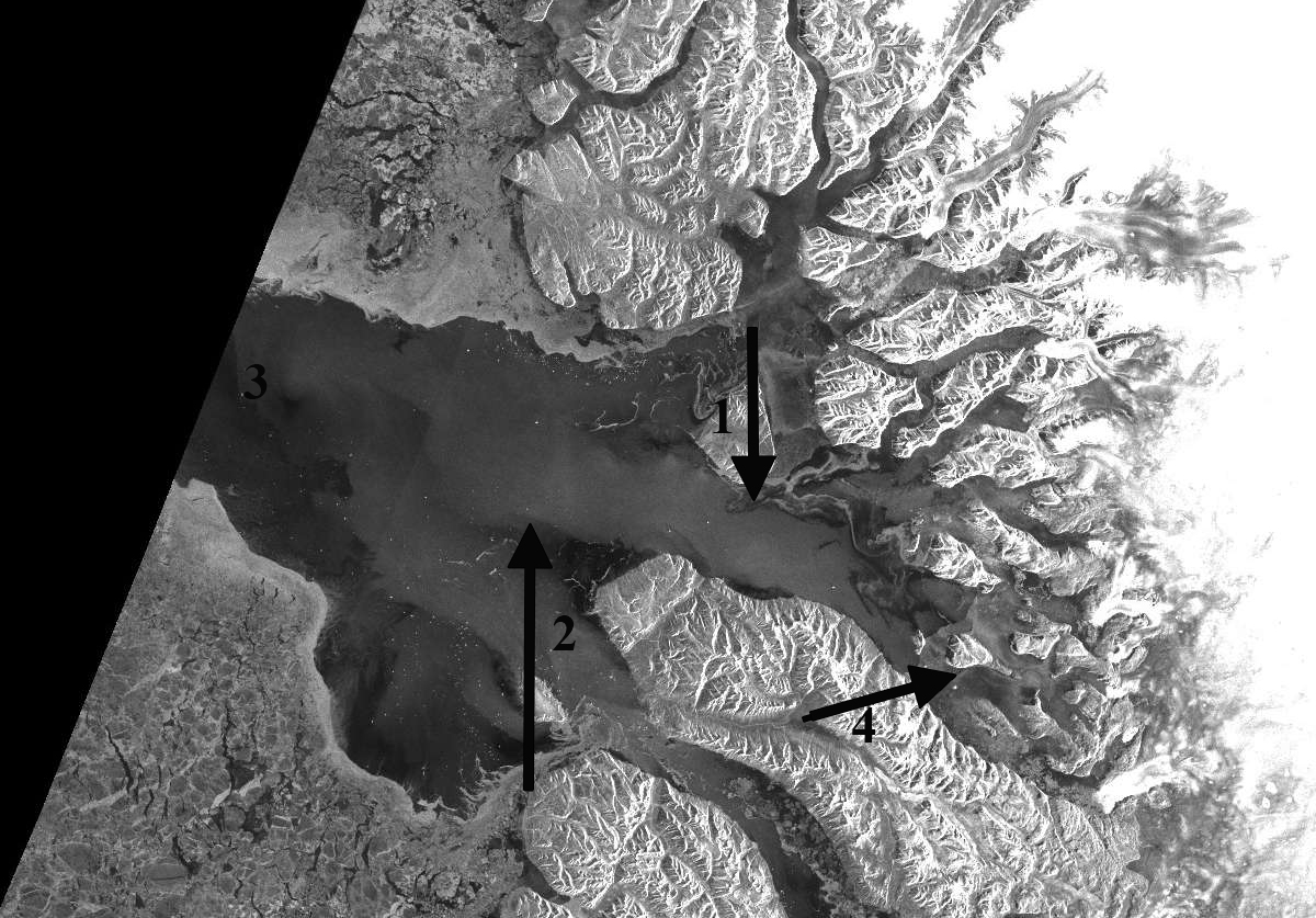
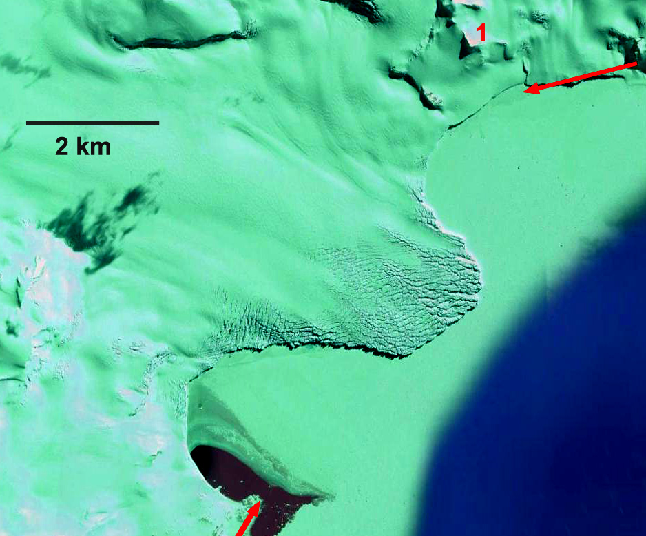
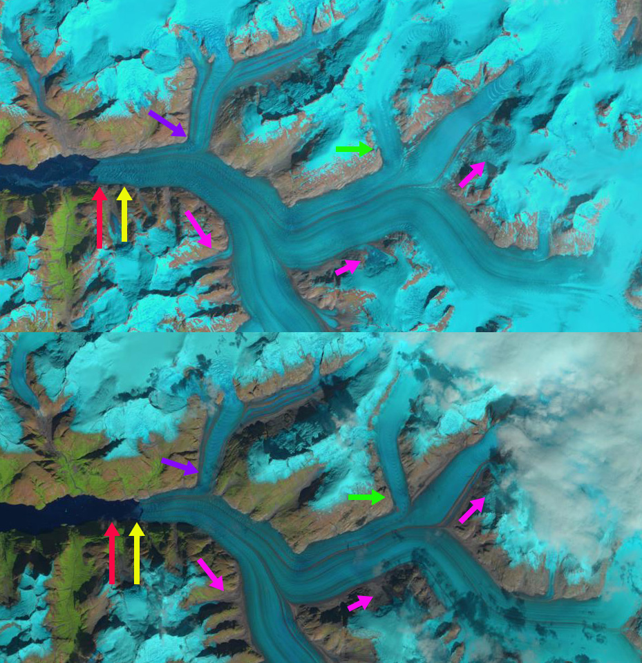
The main terminus has retreated 800 meters from 2001-2013. Here the terminus has pulled back from the tip of the peninsula on the west side of the terminus and is currently at a narrow point.  The eastern terminus has retreated to its junction with the main Ampere Glacier a distance of 1400 m.  Berthier et al (2009) had noted thinning around the Lapperent Nunatak of 150 to 250 m, purple arrows indicate this location of thinning.  Above the current main terminus the valley widens again to the junction with the location of the eastern terminus.  It seems likely the main glacier will retreat north until there is a single terminus north of the southern end of Lapparent Nunatak. Lapparent Glacier was formerly joined with the Ampere Glacier’s eastern outlet.  The comparison of  Landsat imagery from 2001 and 2013 indicate widespread thinning and deglaciation of this glacier.  In 2001 Lapparent Glacier merges with the east terminus of Ampere Glacier at the red arrows with a medial moraine evident.  By 2013 the eastern arm has narrowed from 1100 m to 500 meters and retreated 2100 m in 12 years. The result is less ice flow over a bedrock step just above the terminus. This continued thinning since 2001 will lead to further retreat of the glacier. There is no calving and the rate of retreat will decline. A 2009 Landsat image 2009 and 2013 Google Earth image indicate icebergs stranded in the lake by Lapparent Glacier and the eastern outlet indicating glacier lake drainage lowering the level.

ampere-hd

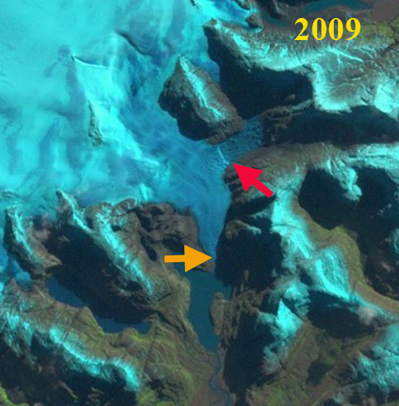
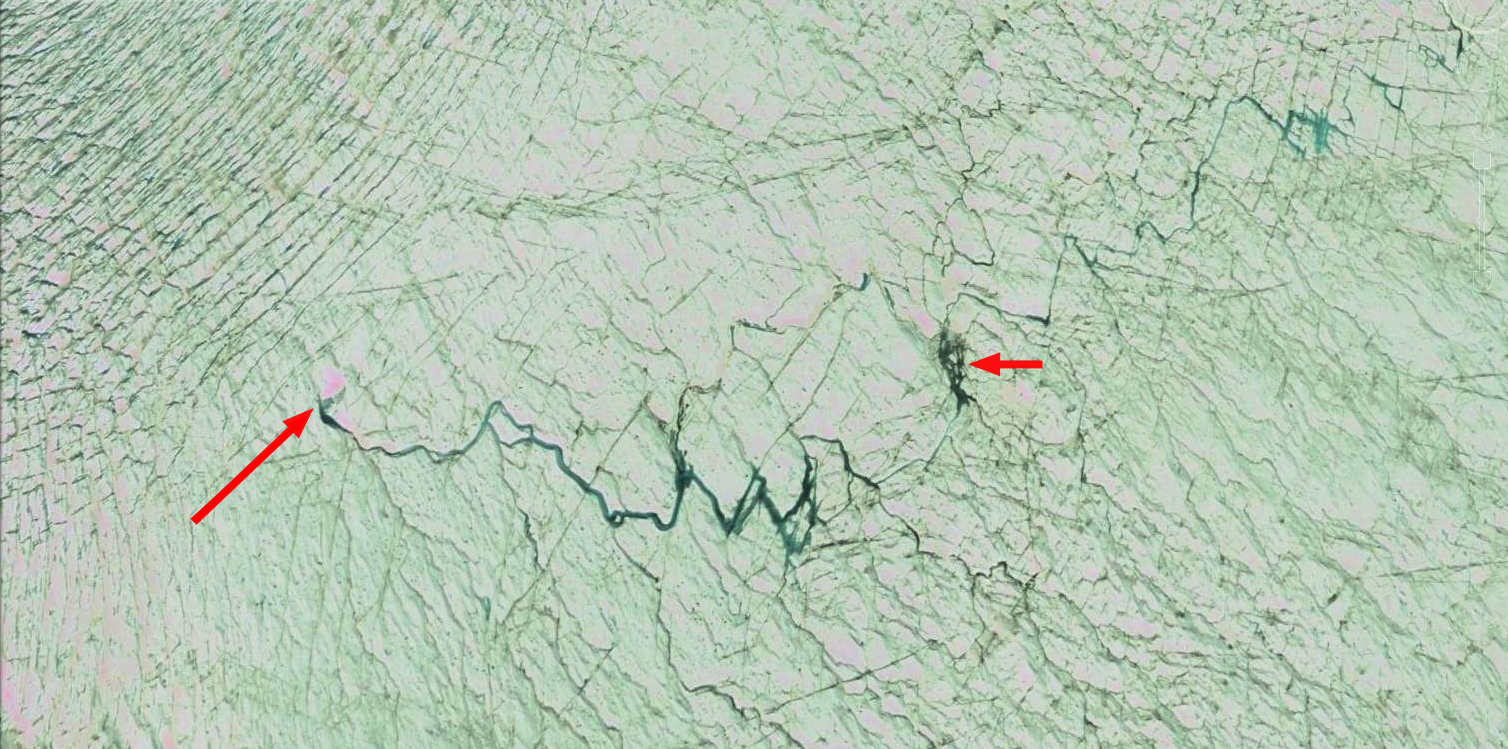
2009 Landsat image icebergs evident in lake in the upper right.

ampere ge

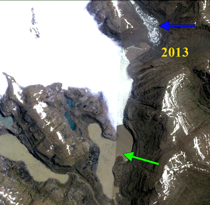
2013 Google Earth, icebergs at blue arrow.  Highly turbid water in proglacial lakes indicates a recent high flow event.
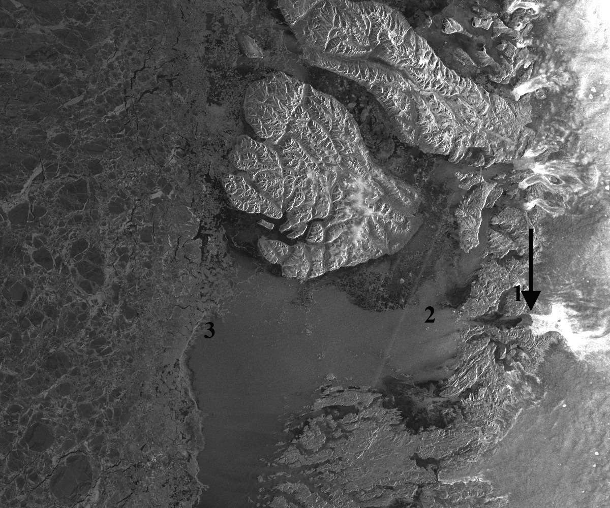
amperre 2016

2016 Landsat image

Pré de Bar Glacier Retreat, Italy

pre de bar compare

Landsat image comparison from 1990 and 2015 of the Pré de Bar Glacier (P).  The adjacent Argentiere Glacier (A) is shown, the red arrow is the 1990 terminus, the yellow arrow the 2015 terminus and the purple dots the snowline. Retreat from 1990 to 2015 was 

Pré de Bar Glacier is a glacier on the east side of Aiguille de Triolet and south side of Mont Dolent. This is a steep valley glacier that experienced a large retreat during the first half of the 20th century, then advanced from the 1960’s-1980’s, before beginning a retreat again in 1990, that has continued to 2015. In the Landsat images above the 1990 terminus extended approximately 600 m beyond the base of an icefall, forming a substantial low slope terminus lobe.  By 2015 this lobe below the icefall had disappeared and the terminus is now at the base of the icefall, with a net retreat of 550 m since 1990.  With the retreat increasing during each five year increment according to WGMS from 1990-2010 and image analysis here from 2011-2015. The retreat is measured each year by the Italian Glacier Committee  and reported to WGMS.  The New Italian Glacier Inventory that has just been released has reports on each region of glaciers in Italy. For the Glaciers of Aosta Valley it is observed that there are 192 glaciers about 21% of Italy’s total, covering 133.7 square kilometers, 24% less than a half-century ago. This amazing inventory was completed by the Earth Science Department of the University of Milan’s Glaciology staff, led by Claudio Smiraglia and Guglielmina Diolaiuti. On page 91 of the Aosta Chapter is a series of images of Pré de Bar from 1897, 1993 and 2012. The main change from 1993 to 2012 is the loss of the terminus lobe below the narrow icefall.

pre de bar historic

Figure from the New Italian Glacier Inventory of Pré de Bar Glacier in 1897, 1993 and 2012

Berthier et al (2014) mapped ice thickness changes in this region from 2003 to 2012 using the Pléiades satellites. They identify a negative Mont Blanc region wide mass balance of glaciers of -1.04 m/year for the 2003-2012 period.  On Pré de Bar Glacier their figure below indicates at least 5 m thinning across nearly the entire glacier, with more than 25 m of thinning in the terminus region below the icefall.  This dramatic thinning largely driven by increasing summer melting. Bonnano et al (2012) identified a long term retreat rate of 3 m per year for the glacier.  However, retreat from 1990 to 2015 is 22 m/year, the WGMS indicates retreat of 404 m from 1990-2010, a rate of 20 m/year.  The rate of retreat incireased from 16 m/year in the 1990’s to 24 m/year in the 2000’s.  The thinning identified by Berthier et al (2014) up to 2012 high on the glacier suggests this will continue.  Note in the image below  from Bonnano et al., (2012) of Pré de Bar Glacier the amount of firn exposed above the ELA particularly on the two easternmost feeders, and the 2015 Landsat image indicates the annual ELA is closer to the end of the black arrows in that image than the red line from 2000.  The pattern of thinning is similar to that of nearby Lex Blanche Glacier, and Glacier d’Argentiere, but Mer de Glace has a much larger relatively low slope ablation zone section with high thinning.

The meltwater runoff from this glacier feeds the Dora Baltea River and eventually the Po River.  The Aosta Valle region hosts extensive hydropower along this drainage including the Avise, Champagne,Nus, Montjovet, Isollaz, Chatillon, Verras, Hone and Ivrea.

mont blanc thinning

Figure from Berthier et al (2014) indicating thinning of Mont Blanc Glacier 2003-2012, Pre de Bar Glacier noted with blue arrow.

Pre-de-Bar
Pre de Bar Glacier in 2000 showing the ablation zone, accumulation zone, ELA, glacier front this is from Bonnano et al (2012)


Where is the snow at Nup La, 5850 m, West Rongbuk Glacier?

nup la 1516

Landsat image from January 4, 2016 indicating the actual Nup La (N).  Purples dots is the snowline. Green arrows are expanding bedrock exposures and pink arrow a specific rock know amidst the glacier.

Nup La at 5850 m is on the Nepal-China border and is the divide between the West Rongbuk Glacier and the Ngozumpa Glacier.  The pass should be part of the accumulation zone of both glaciers.  In recent years including currently this has not been the case, this past Christmas was not a white one at the pass.  Our attention is often focused on the more easily viewed terminus of a glacier, and both of these glaciers are retreating. The changes higher on the glacier can have more far reaching implications. Bolch et al (2011) observed strong thinning in the accumulation zone on nearby Khumbu Glacier, though less than the ablation zone . This can only happen with reduced retained snowpack particularly in winter.  This has occurred with increasing air temperatures since the 1980’s. Mean annual air temperatures have increased by 0.62 °C per decade over the last 49 years; the greatest warming trend is observed in winter, the smallest in summer (Yang et al., 2011). The glaciers in the area are summer accumulation type glaciers with 70% of the annual precipitation occurring during the summer monsoon. There is little precipitation early in the winter season (November-January). The limited snowpack with warmer winter temperatures have led to high snowlines during the first few months of the winter season in recent years. Here we examine Landsat images from 1992 to 2016 to observe changes in the snowline during the early winter period.

In January of 2016 the snowline is at 6100 m, which is well above Nup La and the divide between West Rongbuk and Ngozumpa Glacier.  The green arrows indicate three areas of expanding bedrock exposure occurring over the last 15 years.  This indicates thinning in this region of 5700-6000 m, which should typically be the accumulation zone.  In December 2015 three works prior to the 2016 image the situation is the same.  In November 2014 the snowline is lower at 5750 m.  In 1992 the snowline is at 5600 m, and the bedrock areas at the green arrows are reduced from above.  In November 2000 the snowline is at 5450 m and in November 2001 it is at 5600 m.  In all images prior to 2012 the snowline does not reach the region around Nup La above 5700 m during the early winter period.  In recent years the snowline has remained high, above 5700 m, significantly into the winter season almost every year, and in 2015/16 remains high three months into the winter season. This is an indication of an extended period after the summer monsoon, in which not only is snow not accumulating, but ablation can occur mostly via sublimation at elevations of Nup La. The thinning resulting has caused the expansion of bedrock areas at the green arrows and at the pink arrow.

nup la region
Google Earth image of the region indicating Nup La (N), Wests Rongbuk Glacier (WR), Rongbuk Glacier (R), Ngozumpa Glacier (Ng) and Khumbu Glacier on Mount Everest (K)

nup la dec2015
December 2015 Landsat image indicating the actual Npu La (N).  Purples dots is the snowline. Green arrows are expanding bedrock exposures and pink arrow a specific rock know amidst the glacier.

nup la 11202014
November 2014 Landsat image indicating the actual Npu La (N).  Purples dots is the snowline. Green arrows are expanding bedrock exposures and pink arrow a specific rock know amidst the glacier.

nup la oct92
October 1992 Landsat image indicating the actual Npu La (N).  Purples dots is the snowline. Green arrows are expanding bedrock exposures and pink arrow a specific rock know amidst the glacier.

nup la oct2001
November 2000 Landsat image indicating the actual Npu La (N).  Purples dots is the snowline. Green arrows are expanding bedrock exposures and pink arrow a specific rock know amidst the glacier.

nup la 10152000
November 2001 Landsat image indicating the actual Npu La (N).  Purples dots is the snowline. Green arrows are expanding bedrock exposures and pink arrow a specific rock know amidst the glacier.

nup la 2014
Google Earth image indicating flow paths at Nup La.


Balmaceda Glacier Retreat, Chile Releases Island

balmaceda compare

1986 and 2015 Landsat images of the Balmaceda Glacier, Chile region.  Red arrow indicates 1986 ice front, yellow arrow 2015 ice front and purple arrow a tributary that has detached.

Balmaceda Glacier (Felicia Glacier) is at the southeastern end of the Southern Patagonia Ice Cap (SPI) field and drains into the Serrano River.  There is another glacier referred to as Balmaceda  that descends steeply almost to the shores of Fiordo Ultima Esperanza, hence Felicia Glacier will be used here.  Willis et al (2012) observed that between February 2000 and March 2012, indicate that SPI is rapidly losing volume, that thinning extends to the highest elevations.  The mass balance loss is occurring at a rate of −20.0 ± Gt/year, which is +0.055 mm/year of sea level rise. The retreat is driven by increasing calving rates from the 1975-2000 to the 2000-10 period (Schaefer et al, 2015). The pattern of retreat is consistent between these glaciers and the region as noted by Davies and Glasser (2012),  annual rates of shrinkage in the Patagonian Andes increased in  from 0.10% year from 1870-1986, 0.14% year from 1986-2001, and 0.22% year from 2001-2011. These losses have led to retreat such as at Glaciar Marconi and Glacier Onelli

In 1986 the glacier terminated on an island in that acts as pinning point stabilizing the glacier front.  The calving front is over 2.5 km wide. By 2000 Landsat imagery indicates the glacier has retreated from the island with the greatest retreat on the north side.  By 2013 the glacier has receded into a narrow western arm of the lake, the snowline is at 600 m. By 2015 a southern tributary has separated from the main glacier at the purple arrow. The terminus at the yellow arrow is 1 km from an increase in surface slope indicating a rise in bedrock that may be the inland margin of the lake. The retreat from 1986 to 2015 is 2100 m and the current calving front is 1.2 km wide.  The snowline in 2015 is at 1000 m is quite high.  De Angelis (2014) notes the ELA for this glacier at 690 m.  Above the snowline the linear wind sculpted features oriented west to east indicate the ferocious winds of the region Schaefer et al (2015) note the exceptional accumulation rates in the region

The Balmaceda Glacier drains into the Serrano River, the headwaters being Del Toro Lake on the southern boundary of Torres del Paine National Park.  The river is home to numerous giant Chinook salmon which can weigh up to 35 kg with fishing season from June to December.  Chinook salmon have just recently started populating rivers in Chile and Argentina. Fish hatcheries in southern Chile release thousands of Chinook smolts. The introduced Chinook originate from tributaries of the Columbia River of Washington and Oregon.

balmaceda 2000

2000 Landsat Image

balmaceda 2013

2013 landsat image

balmaceda 2015

2015 Landsat image the purple dots are the snowline which at 1100 m is quite high.  Also note the long wind drift features extending west to east above the snowline.


What is Up in Disko-Uummannaq Bay Greenland January 9-16, 2016

@TenneyNaumer contacted Alun Hubbard, Jason Box and I with an astute observation last evening. “But what I am getting at is that in general the temperature anomalies over the region of Jakobshavn have been high in the last few days, and I spotted weird temperatures off the coast via Climate Reanalyzer (which is seriously low resolution).  I just checked with the manati satellite (also seriously low resolution), and it seems some sort of event has taken place.”

Following up on what are typically good observations from Tenney I looked at the Radarsat-2 and Sentinel-1 imagery posted by the Danish Meteorological Institute.  Weather records from automatic weather stations in the region from PROMICE and the surface mass balance model results for the week from Polar Portal.

It is evident from the PROMICE weather records on the ice sheet just south of the Disko Bay region that temperatures have been exceptionally high since January 5th and atmospheric pressures have been high since January 9th.  The Polar Portal mass balance model indicates some actual declines/ablation in the last week. This is more likely sublimation from föehn conditions than actual melt.  The real changes are in the sea ice fronts and ice in the coastal inlets illustrated by MODIS. Below are images from January 9, 11, 13 and 16 for Disko Bay and January 9, 13 and 16 from Uummannaq Bay.

The arrow at location 1# is an area of sea ice across the fjord in front of Jakobshavn Glacier on January 9, that disappears by January 13. Location #2 is at the fjord mouth and location #3 is at the sea front south of Disko Island on January 9.  There is no real cloud cover evident in any of images.  Maybe low level fog in places. By January 11th a plume is sweeping from Point 2 towards Point 3. Notice the sea ice in the fjord disappears by January 13th and the ice front is pushed back in a concave fashion at Point #3. This indicates a clear push of water driving sea ice offshore. The Ilulissat Fjord mouth lack of ice is also evident in Webcam images from 1-16-16 and 1-17-16 at the Hotel Arctic, last images below with two boats plying the open water. on the 16th and icebergs clogging the fjord mouth on the 17th.  The Sentinel-1 image from January 16th shows a significant flushing of icebergs from Ilulissat Fjord, pointed out by black arrows.  This image has better clarity and with the icebergs scattered through the plume, indicate more clearly the plume is a water source change event, even if wind driven. The iceberg plume in the fjord has a brighter aspect due to the varied surface aspect-reflectance and has expanded down fjord.  The event must be due to or enhanced by strong offshore winds and Ruth Mottram (@ruth_mottram) indicates there was at least one föehn event this week. The plume includes bergs from the ice melange in front of Jakobshavn has been largely removed, which can have implications for calving and frontal velocity. Moon et al, (2015). indicate the role that a rigid ice melange has on the calving and frontal velocity of tidewater outlet glaciers in Greenland.

In Uummannaq Bay a very similar sequence plays out, note on January 9 the sea ice connecting islands near #4.  By January 13th the ice at location #4 is gone.  The ice front is now at location #3, which on January 9th was well into the ice pack.  Again we have a clear push of water leading to a concave sea ice front that is pushed well offshore. Icebergs can be seen amidst plume on January 16th, the plume opacity and size has diminished since January 13th.

In both of the January 13th images there is a plume leading to the concave sea ice front, the question being is this sediment laden water, with the resultant higher reflectivity or is it a combination of a surface water change from wind or a combination. We had questioned if the plume had any sediment origin initially. Its widespread nature and persistence suggested not.  Aeration was another suggestion.  Jason Box suggests that the opaque water plume leading to the developing polyna is driven by the strong offshore winds and the opaque whitening is capillary waves on the sea surface. Examples of identification of observed high backscatter from offshore winds are from Monaldo and Beal (1998) and Li et al, (2007) The ice must in part be driven back by a surface water push. You can see icebergs in sections of the plumes closer to shore suggesting this is a surface near surface phenomenon. This is a short term event.  However, it could have broader implications,  in this case the ice melange in front of Jakobshavn has been removed, and probably from in front of other glaciers, which will impact near term calving rates. I have incorporated many insights from the community and welcome more.

20160109s01disko

RADARSAT-2 IMAGE FROM Disko Bay  1/09/2016

20160111rs02disko

RADARSAT-2 IMAGE FROM Disko Bay  1/11/2016

20160113rs02disko

RADARSAT-2 IMAGE FROM Disko Bay  1/13/2016

20160116disko

Sentinel-1 imagery from 1-16-16 of Disko Bay-notice expanded brightness area in the fjord by #1.

20160109s01uummann

 Sentinel 1 imagery of Uummannaq Bay 1/09/2016

20160113rs02umman

RADARSAT-2 IMAGE FROM Uummannaq Bay MODIS 1/13/2016

20160116s01uumann

Sentinel 1 imagery of Uummannaq Bay  1/13/2016 plume size and opacity diminishing. 

illusiat webcam 1-16-2016

Ilulissat Fjord mouth webcam view 1-16-16.

ilulissat webcam11-17-16

Ilulissat Fjord mouth webcam view 1-17-16.

Murchison Glacier, New Zealand Rapid Retreat Lake Expands 1990-2015

murchison compare

Murchison Glacier change revealed in Landsat images from 1990 and 2015.  The red arrow indicates 1990 terminus location, the yellow arrow indicates 2015 terminus location and the purple arrow indicates upglacier thinning.

Murchison Glacier is the second largest in New Zealand.  The glacier drains south in the next valley east of Tasman Glacier and terminates in a lake that is rapidly developing as the glacier retreats. The lower 6 km section  is debris covered, stagnant, relatively flat and will not survive long. There was not a lake in the 1972 map of the region.  In 1990 the newly formed lake was limited to the southeast margin of the terminus . From 1990 to 2015 the terminus has retreated 2700 m. A rapid retreat will continue as 2010, 2013 and 2015 imagery indicate other proglacial lakes have now developed 3.5 km above the actual terminus. These lakes are glacier dammed and may not endure but do help increase ablation, and in the image below show a glacier that is too narrow to provide flow to the lower 3.5 km. The demise of the lower section of this glacier will parallel that of Tasman Glacier.  The expanding lake will continue to enhance the retreat in part by sub-aqueous calving noted by Robertson et al (2012) on nearby glaciers. The increased retreat has been forecast by the NIWA and Dykes et al (2011). The glacier still has a significant accumulation area above 1650 m to survive at a smaller size.  The ongoing retreat is triggered by warming and a rise in the snowline in the New Zealand Alps observed by the NIWA. Notice the changes upglacier indicated at the purple arrows above, where tributary flow has declined, bedrock areas in accumulation zone have expanded and the snowline is higher.  Gjermundsen et al (2011) examined the change in glacier area in the central Southern Alps and found a 17% reduction in area mainly from reductions of large valley glaciers such as Murchison Glacier.

mucrhison terminus reach compare

Terminus reach of Murchison Glacier in Google Earth images from 2007 and 2013.  Note expansion at pink arrow on the terminus lake and the development of proglacial lakes 3.5 km upglacier at blue arrows.

The Feb. 2011 earthquake near Christchurch led to a major calving event of a portion of the rotten stagnant terminus reach of the Tasman Glacier. There was no evident calving event from Murchison Glacier.This has led to increased exposure of bedrock high on the glacier and reduction of tributary inflow noted at purple arrows.

Murchison Glacier drains into Lake Pukaki,a along with Hooker, Mueller and Tasman Glacier, where water level has been raised 9 m for hydropower purposes. Water from Lake Pukaki is sent through a canal into the Lake Ohau watershed and then through six hydropower plants of the Waitaki hydro scheme: Ohau A, B and C. Benmore, Aviemore and Waitaki with a combined output of 1340 MW.  Meridian owns and operates all six hydro stations located from Lake Pūkaki to Waitaki. Reductions in glacier area in the watershed will lead to reduced summer runoff into the Lake Pukaki system. Below the Benore Dam is pictured,.  Interestingly salmon have been introduced into the Waitaki River system for fishing near its mouth. Benmore Lake itself is an internationally renowned trout fishing spot, providing habitat for both brown trout and rainbow trout.

benmore dam

Google Earth Image with Benmore Dam in foreground and Benmore Lake.  This hydropower system is fed by a canal from Lake Pukaki which in turn is fed by Murchison Glacier.


Hooker Glacier Retreat, 1990-2015

hooker compare

Glacier change revealed in Landsat images from 1990 and 2015.  Mueller Glacier (M) and Hooker Glacier (H).  The red arrow indicates 1990 terminus location, the yellow arrow indicates 2015 terminus location and the purple arrow indicates upglacier thinning.

Hooker Glacier parallels the Tasman Glacier one valley to the west draining south from Mount Hicks and Mount Cook.  Hooker Glacier is a low gradient which helps reduce its overall velocity and  a debris covered ablation zone reducing ablation, both factors increasing response time to climate change  (Quincey and Glasser 2009). Hooker Lake which the glacier ends in began to from around 1982 (Kirkbride, 1993).  In 1990 the lake was 1100 m long (Figure 11.2).  From 1990 to 2015 the lake expanded to 2300 m, with the retreat enhanced by calving. The 1200 m retreat was faster during the earlier part of this period (Robertson et al.,2013).

hooker-mueller 1972 map

Map of the region in 1972 indicating the lack of proglacial lakes at the end of Mueller, Hooker and Tasman Glacier

The lower 3.4 km of the glacier has limited motion.  Robertson et al, (2012)  suggest the retreat will end after a further retreat of 700-1000 m as calving will decline as the lake depth declines.  The peak lake depth is over 130 m, with the terminus moving into shallow water after 2006 leading to declining retreat rates (Robertson et al (2012).Gjermundsen et al (2011) examined the change in glacier area in the central Southern Alps and found a 17% reduction in area mainly from reductions of large valley glaciers such as Hooker Glacier. Based on the nearly stagnant nature of the lower glacier and the diminished ice flow from above indicated by debris cover expansion at the purple arrow, it seems likely the retreat will continue well beyond the end of the lake but at a diminished rate.

Hooker Glacier drains into Lake Pukaki,a along with Murchison, Mueller and Tasman Glacier, where water level has been raised 9 m for hydropower purposes. Water from Lake Pukaki is sent through a canal into the Lake Ohau watershed and then through six hydropower plants of the Waitaki hydro scheme: Ohau A, B and C. Benmore, Aviemore and Waitaki with a combined output of 1340 MW.  Meridian owns and operates all six hydro stations located from Lake Pūkaki to Waitaki. Reductions in glacier area in the watershed will lead to reduced summer runoff into the Lake Pukaki system (see image below)

hookder 2006-2013

Comparison of Hooker Glacier terminus area in 2006 (red arrow) and 2013 (yellow arrow) in Google Earth. Blue arrow indicates icebergs in 2006.

pukaki hydro

Hydropower projects below Lake Pukaki

Endurance Glacier, Elephant Island Retreat

endurance glacier compare

Landsat comparison from 1990 and 2015 of Endurance Glacier, Elephant Island-Embayment development east and west side of calving terminus. 

Endurance Glacier is the main outlet glacier of this heavily glaciated island of the South Shetland Islands. The name of the island comes from the numerous elephant seals. The name of the glacier comes from the Ernest Shackleton and his crew from the Endurance reaching the island in 1916 after a journey in open boats, following the loss of their ship Endurance in Weddell Sea ice.  Amazingly 28 men somehow survived the trip to Elephant Island. The name is also appropriate as it takes real endurance to visit and observe the glacier as is evident in the lack of observations on this glacier. I have been waiting since the launch of Landsat 8 in 2013 for a reasonably clear image of this obviously cloudy area. The December 16th, 2015 image is that image. here we examine the changes in this glacier from 1990 to 2015 using Landsat images. Endurance Glacier has 6 km wide calving front facing the open ocean. The glacier is heavily crevassed in the center near the calving face. This glacier must be exposed to as much wave action as any glacier in the world, since it lacks sea ice protection from November-May.

elephant island

 Elephant Island, South Shetland Islands

In 1990 the calving front has a slight convexity with the terminus extending parallel to the coast from the red arrows. A specific nunatak is Point 1, and is 1.4 km from the calving front. By 2001 embayments have begun to develop on the east and west end of the calving front. By 2015 the calving front has a pronounced convex center with two substantial embayments on the east and the west. Point 1 is now 700 m from the calving front. The embayment adjacent to this indicates a retreat of 500-1000 m across a 2 km ice front. The western embayment is larger 2.25 km wide with the front having retreated 1000 to 1500 m. The increasing exposure of the central terminus tongues to wave action and ocean water, should lead to its loss in the near future. This is evident in the Google Earth image below. This glaciers retreat is less than glaciers on South Georgia such as Neumayer and Hindle Glacier.

elephant island 2000
2001 Landsat image

elephant island ge

Google Earth image from 2014 note convex center tongue, embayments east and west and heavy crevassing.


Orpissuup Tasia Glacier slowdown, SW Greenland

transects_chart_1985-2013

Tedstone et al (2015) Figure 3 illustrates the widespread velocity decline along three transects. 

Pelto et al (1989) after a field campaign we mounted in 1985 and 1986 on Jakobshavns Glacier noted that the velocity was essentially the same in the summer of 1964, 1976, 1978, 1985 and 1986.  Further we observed that the agreement between surface mass-balance and volume-flux calculations, suggested that “Jakobshavns Isbrae: is almost in a state of equilibrium”. The point of the study was to establish a baseline of velocity before the anticipated acceleration due to warming. This acceleration due to warming happened beginning in 1992 from 20 m/day at the calving front in 1985 to 46 m/day in 2012, comparing the same locations the annual speed increase was 282% from 1992 to 2012 (Joughin et al 2014).  The Jakobshavns Isbrae is a tidewater glacier, just south of the glacier the margin of the ice sheet is dominated by a land terminating section that has a different dynamic response to warming.

Tedstone et al (2015) in a paper published in Nature in October noted a decadal reduction in glacier velocity for a land terminating region of the Greenland Ice Sheet. This slow down occurred despite a 50% increase in meltwater production. This is emphasized in the figure above indicating the changes along three transects from green earlier to purple later years.  A glacier inhabits a particular topographic environment that establishes the basic flow field. Climate change can affect glacier flow by increasing ice melt, which leads to ice thinning  and a consequent reduction in force generating ice deformation and flow.  This same ice melt can deliver meltwater to the base of the ice sheet, which can lead to short term increases in basal water pressure that will drive acceleration, the acceleration tends to be short lived.  The overall impact of these competing forces is what this study indicates, that just as is the case on alpine glaciers thinning resulting from more melt leads to velocity reductions as a more efficient hydrologic system develops reducing basal water pressure.  This same process clearly does not apply to calving tidewater outlet glaciers. Here we examine the changes at the terminus, evidence of thinning and location of moulins on the outlet glacier that flows into a series of lakes, Orpuussit Tasia, along Transect B.

transect b landsat compare

Landsat image comparison from 2000 and 2015.

In the comparison of Landsat images above from 2000 and 2015 the expansion of small proglacial lakes is evident at each red arrow, #2 has the greatest expansion.  At the yellow arrows thinning is evident at a small lake that is fed by glacier runoff giving it a green sediment laden color, and by 2015 no longer receives meltwater as the ice sheet has thinned below the watershed divide, yielding clearer water which appears darker.  The expansion of the end of the medial moraine also indicates thinning.  Four bedrock areas emerging from the ice have much greater prominence in 2015 than 2000 purple arrows. This is modest thinning and retreat compared to the Jakobshavn and other large outlet glaciers to the north. The first image below indicates the terminus with red dots in a Google Earth image. The terminus as the proglacial lake #2 is pinned on a two bedrock prominences which should slow retreat. Proglacial lake #3 does not have an evident pinning point, and should retreat back towards the peninsula to the south in the near future. The second image below indicates the supraglacial streams and moulins in a small area of this glacier. The linear nature of many streams indicate they are occupying former crevasse features. Just as in the 1980’s little of the runoff reaches the terminus at the surface, almost all is directed to the base via moulins. Tedstone et al (2015) found that velocity did increase in summer, but declined more in the winter.  NASA Landsat and Nasa Earth Observatory provides several excellent figures and explanation of the process in the study area.

.transect b

Google Earth image indicating ice sheet margin in 2012, red dots.

transect b moulins

Google Earth image indicating surface streams and locations of two moulins. 

Lex Blanche Glacier Recession, Mont Blanc Massif, Italy

lex blanche compare

Lex Blanche Glacier (Lb) comparison in a 1990 and 2015 Landsat image.  Red arrow indicates 1990 terminus, yellow arrow the 2015 terminus and the purple arrow a separated tributary. Debris covered Miage Glacier (M) is adjacent. 

Lex Blanche Glacier descends from 3500 m on the southeast flank the Aiguille de Glaciers of the Mont Blanc Massif into the Vale Veny of Italy. The glacier is adjacent to Miage Glacier (M). The glacier advanced over 700 m from 1970 to 1990. In 1990 the glacier extended to the base of a steep slope and turned north to terminate at 1980 m. By 2001 the glacier has retreated up a steep slope to near where the 1970’s advance had begun.  By 2009 and 2011 further retreat has left the terminus just above a particularly steep bedrock slope.  By 2015 the glacier has retreated 1100 m and terminates at 2450 m remaining on a relatively steep slope. The glacier is heavily crevassed a short distance above the terminus suggesting the period of rapid retreat should be ending. A tributary from the north has detached from the main glacier at the purple arrow. In recent warm summers the glacier has retained snowcover above 3150 m.  The mass balance noted in Figure 8  (see below) of a paper by Berthier et al (2014) indicates the thinning is glacier wide but most prominent on glacier tongue.  Berthier et al (2014) used  the Pléiades satellites to identify a negative region wide mass balances of glaciers in the Mont-Blanc area of -1.04 m/year for the 2003-2012 period. The meltwater runoff from this glacier feeds the Dora Baltea River and then the Po River.  Both rivers feature extensive hydropower including the Champagne and Nus hydropower plant on the Dora Baltea  that produce 41 MW.  The retreat of this glacier mirrors that of other glaciers of Mont Blanc including Taconnaz, Bionnassay, Mer de Glace and Tour Glacier.

berthier mass balance lex blanche

Figure 8 from Berthier et al (2014) on glacier wide mass change with thinning in browns, and darker browns greater thinning.

lex blanche 2001

Google Earth image from 2001 indicating the 1990 terminus at red arrow and 2001 terminus at yellow arrow.

lex blanche 2009

Google Earth image from 2009 indicating the 1990 terminus at red arrow and 2009 terminus at yellow arrow.

lex blanche 2011

Google Earth image from 2011 indicating the 1990 terminus at red arrow and 2011 terminus at yellow arrow.  Blue arrow indicates the lowest heavily crevassed region.


Kanchenjunga Glacier, Nepal Volume Losses

kanchenjunga compare
Figure 10-16. Kanchenjunga Glacier (K) from 1991 to 2015, green arrows indicate locations of enhanced supraglacial lakes since 1991. Purple arrow indicates areas of thinning at higher elevations in the region. Location 2 is the main junction area. 

Kanchenjunga Glacier is the main glacier draining west from Kanchenjunga Peak, also listed on maps as Kumbukarni. The glacier is similar to Zemu Glacier flowing east from the same mountain into Sikkim, in the heavy debris cover that dominates the glacier in the ablation zone extending from the terminus for 15 km and an altitude of 5600 m. Identifying the retreat is difficult due to the debris cover. Racoviteanu et al (2015) examined glaciers in this region using 1962 and 2000 imagery. They found area losses of 14% for debris covered glacier and 34% for clean glaciers. The debris covered glaciers terminus response is even more muted indicating why terminus change is an easy measure of glacier change but not always the best. For Kanchenjunga Glacier Racoviteanu et al (2015) indicate the glacier area declined by just 4-8% from 1962-2000.

What is apparent in the Landsat images at the green arrows is the increase from 1991 to 2015 of supraglacial lakes. Also features of thinning are evident in the mid reaches of the glacier, purple arrows, where tributaries have narrowed and detached from the main glacier. A closeup of the main glacier junction 12 km above the terminus indicates the number of large supraglacial lakes. These cannot form in a region where melting does not dominate over glacier motion. The Google Earth image from 2014 of the terminus area indicates a patchwork of moraine cored ice dotted with supraglacial lakes and dissected by the glacial outlet river in the lower 3 km of the glacier. This is clearly not an active portion of the glacier, it is thin not moving and does not fill even the valley floor. An overlay of images indicates the lack of motion. The heavy debris cover has slowed retreat and thinning, however, the lower glacier is poised for an increased rate of retreat with merging of supraglacial lakes, which will lead to further area losses. The Kanchenjunga Glacier is losing volume like all other 41 glaciers examined in detail and linked at the Himalayan Glacier Index page. 

kanchenjunga glacier jct

Google Earth image of the main glacier junction region (2) Supraglacial lakes in the area of at 5200 m. 


kanchenjunga glacier

Google Earth image of supraglacial lakes 2-5 km above the terminus and the region along the north margin of the glacier where the glacier is receding from the lateral moraine. 

kanchenjunga terminus

2014 Google Earth image of terminus reach.  Black arrows indicate ice cored moraine, blue arrow the lowest large supraglacial lake, 2.5 km above the terminus and red arrow the last remnant of ice. 

Dawes Glacier, Alaska Retreat and Harbor Seals

dawes compare
Comparison of 1987 and 2015 Landsat images of Dawes Glacier. Red arrow 1987 terminus, yellow arrow 2015 terminus, pink arrow location where tributaries separated.

Dawes Glacier terminates at the head of Endicott Arm, a 55 km long fjord in southeast Alaska.  Dawes is a major outlet glacier of the Stikine Icefield.  Larsen et al (2007) observed a rapid thinning of the Stikine Icefield and that Dawes was thinning faster than all but Muir Glacier in Southeast Alaska during the 1948-2000 period. During the period from 1891 when first mapped and 1967 the glacier retreated 6.8 km (Molnia,2008). The retreat has been driven by rising snowlines in the region that has driven the retreat of North Dawes, Baird and Sawyer Glacier.

A comparison of 1987 and 2015 Landsat images illustrate recent retreat and thinning of the glacier.  The main terminus retreated 1100 m during this interval, a reduced rate from the previous period from 1978 to 1987 the glacier retreated 2.8 km. Key tributaries at the purple and green arrow each have a 30% decline in width.  At the pink arrows are three tributaries that fed the Dawes Glacier in 1987 and are now detached.  This fragmentation will continue.  The reduced inflow and up glacier thinning is ongoing as will the retreat.  A key mechanism for retreat over the last century has been calving.  The calving rate has declined of late, possibly due to reduced water depth. The 2007 Hydrographic map of the area indicates water depth at the calving front still over 100 m., with a depth of 150 m 1 km down fjord of the terminus (see bottom image). Examination of surface elevation portrayed in Google Earth indicate a relatively sharp rise near the first junction, the surface elevation being at 1400 feet.  The trimline is noted with blue arrows, note how much higher above the ice the tramline is at the terminus than at 1400 feet.  At this point the northern arm would appear to have a bed above sea level and the main arm at least a much shallower bed.  Pelto and Warren (1991) observed the calving rate reduction with water depth in the area.  Note the ogives, curved bands, on the northern arm that form once per year at the base of icefall due to seasonal velocity change. The glacier thinning is continuing, but the retreat rate will decline as the fjord head is approached.  As calving is reduced harbor seals will be disappointed as they like us are drawn to glaciers.

dawes ge 2013 copy

Google Earth image of Dawes Glacier in 2013. Blue arrows indicate trillion and number are elevation in feet.

The Alaska Department of Fish and Game has been monitoring harbor seals in the fjord and noting their use of icebergs and proximal glacier regions. The noted that females travel to pup on the icebergs in the spring and also utilize the are for mating. Because there was little information on where seals that use glacial habitat during pupping and mating season spend the remainder of the year, ADFG attached satellite tags to harbor seals to monitor their movements. In 2008 this data indicated that that adult and sub-adult seals captured in Endicott Arm early summer spent the late summer and fall months in Stephens Passage, Frederick Sound, Chatham Strait,  This study is in part prompted by a decline of harbor seals in the Glacier Bay region where they also utilize icebergs, as NPS biologist Jamie Womble explained at the AGU 2015 meetin

dawes 1978

1978 Landsat image, blue arrow 1978 terminus, red arrow 1987 terminus and 2015 terminus yellow arrow.  Note the improvement in the Landsat imagery.


OPR-O168-FA-07(H11759)