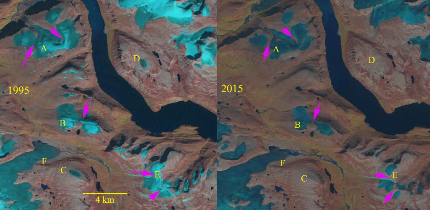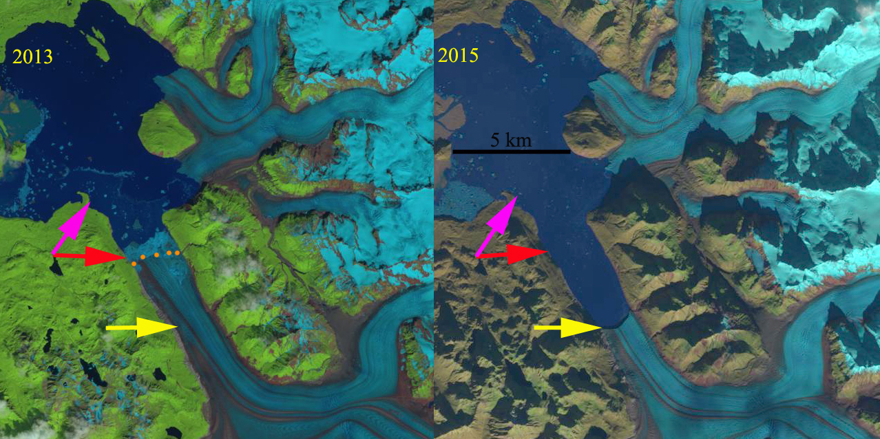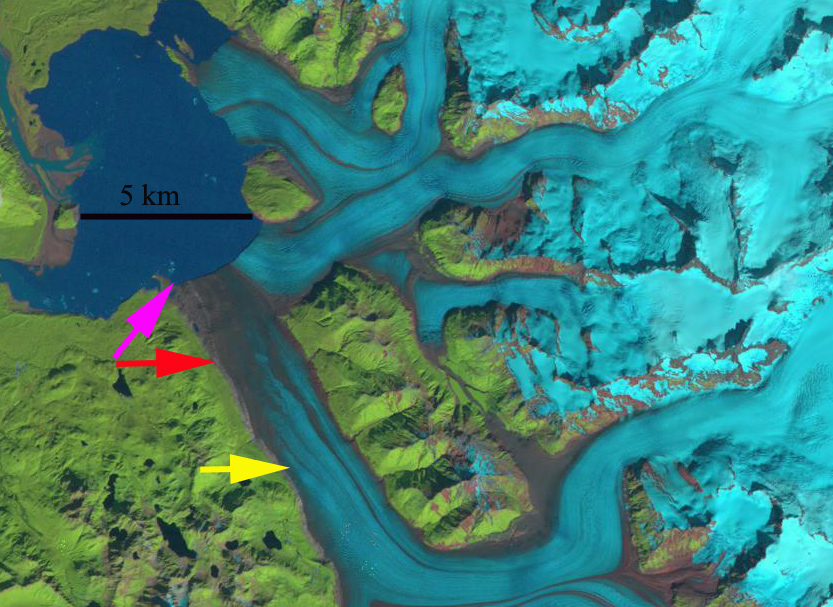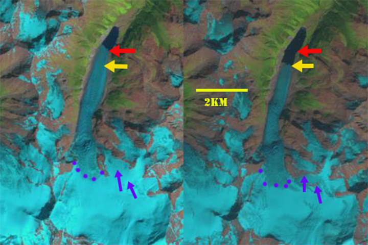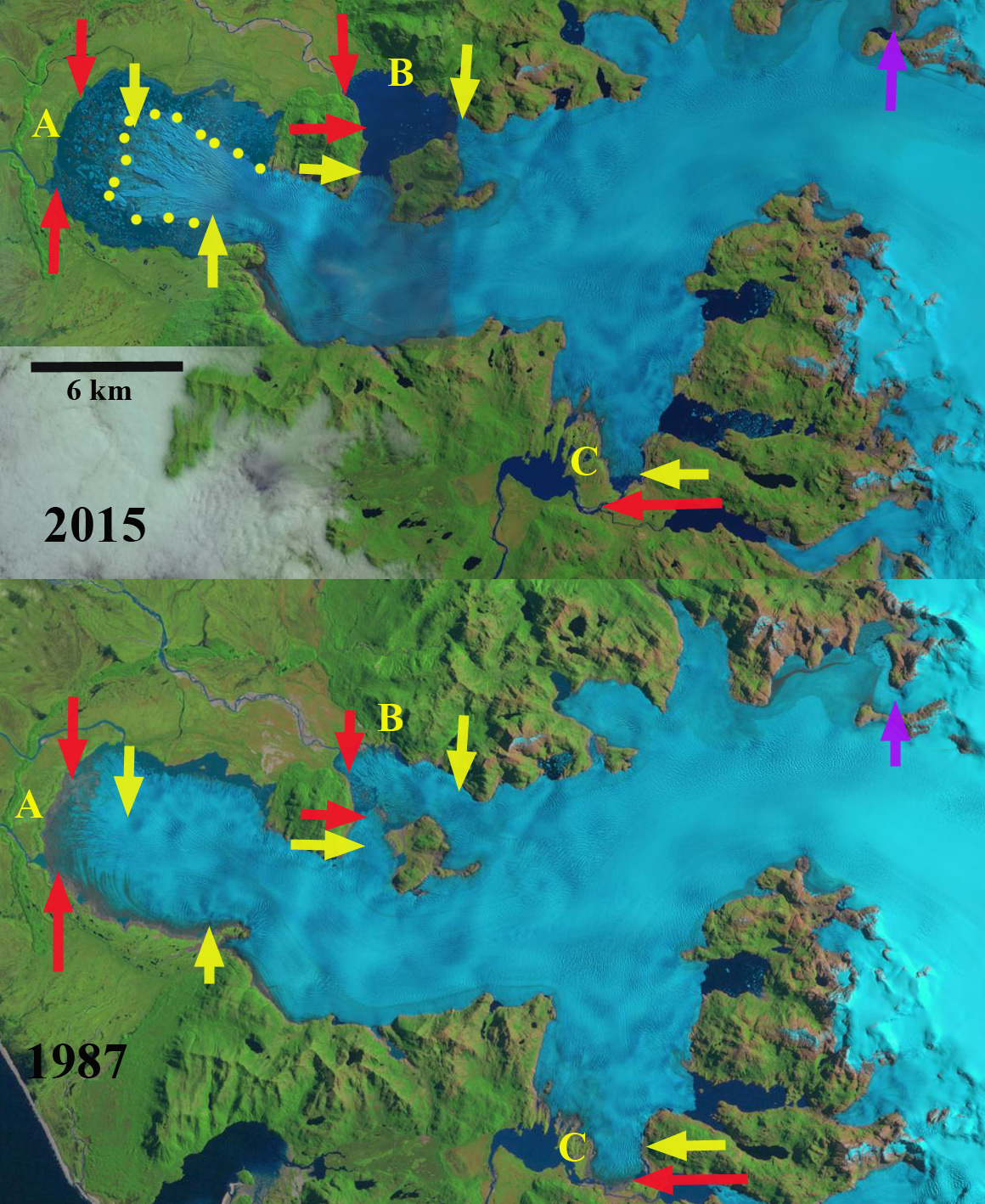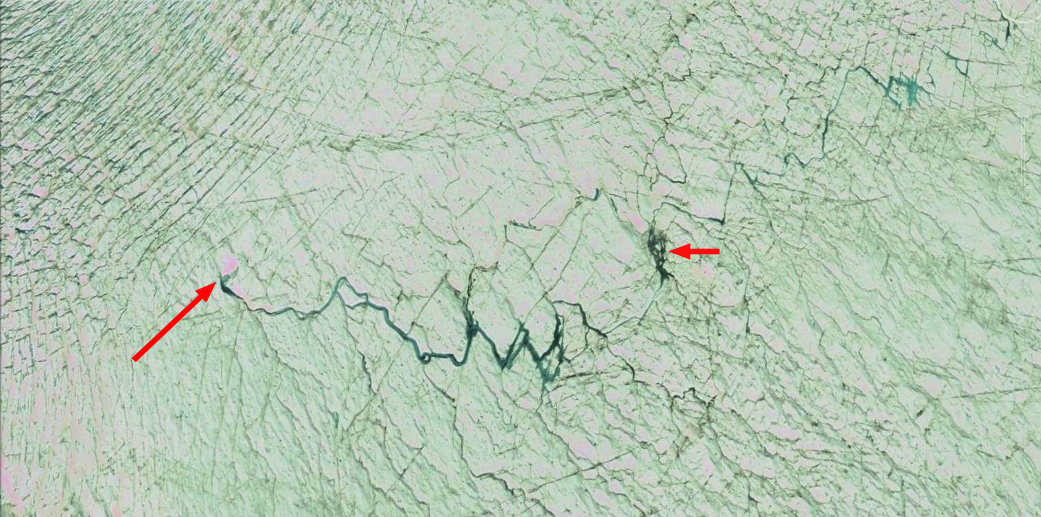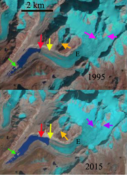
Chubda Glacier comparison in 1995 and 2015 images. Red arrow indicates 1995 terminus location and yellow arrow is 2015 terminus location. Pink arrows indicate areas upglacier of expanding bedrock. Green arrow indicates moraine areas amidst the lake. The orange arrow indicates a secondary glacier.
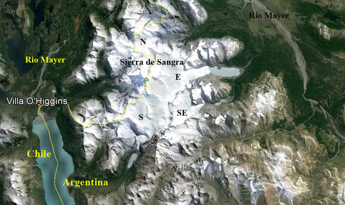
Chubda Glacier, Bhutan drains south from Chura Kang on the Bhutan/China border. The glacier terminates in Chubda Tsho, a glacier moraine dammed lake, Komori (2011) notes that the moraine is still stable and the lake is shallow near the moraine, suggesting it is not a threat for a glacier lake outburst flood. Mool et al, (2001) indicate the glacier was 3.4 km long and 0.3 km wide in the late 1990’s. Jain et al., (2015) noted that in the last decade the expansion rate of this lake has doubled. The glacier feeds the Chamkhar Chu basin which has a proposed 670 MW hydropower project under consideration. Here we examine changes in the Chubda Glacier from 1995 to 2015 with Landsat imagery.
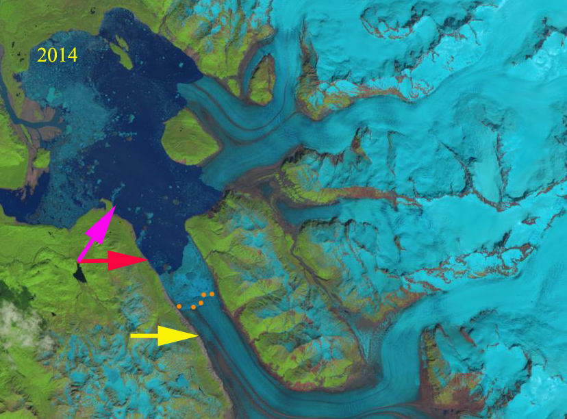
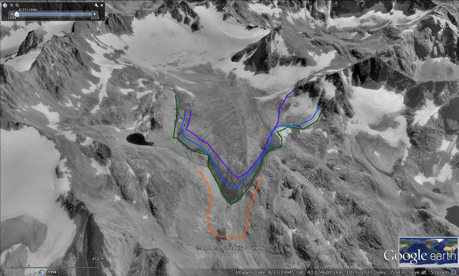
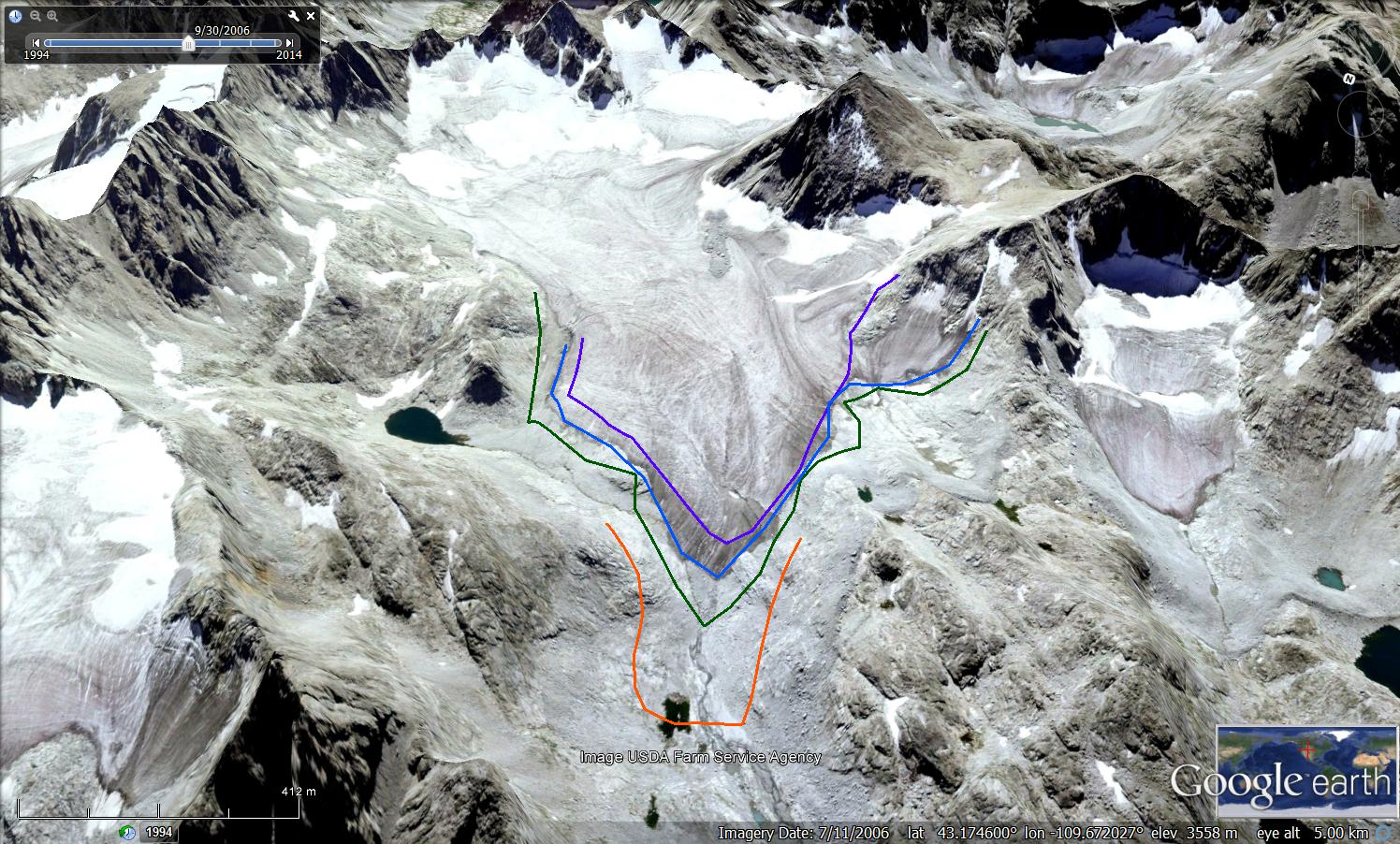
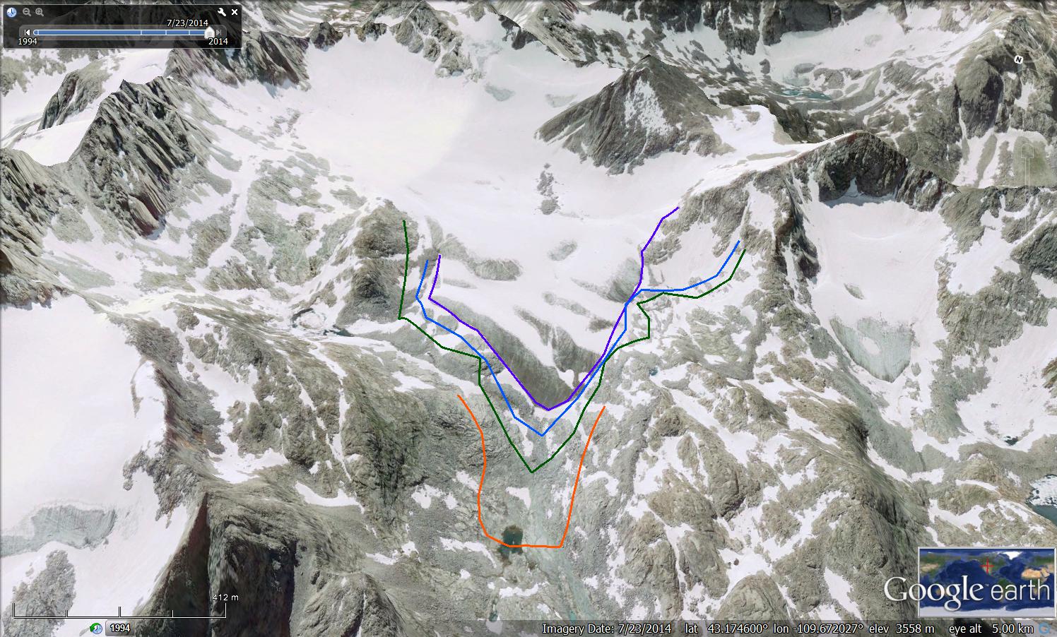
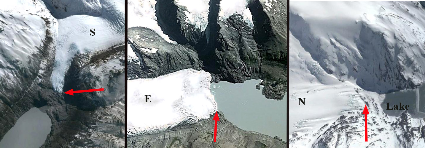
In 1995 Chubda Glacier terminated at the red arrow and there was considerable ice cored moraine remaining in the southern portion of Chubda Tsho, green arrow. The glacier is 700 m wide at Point E and has limited exposed bedrock areas just above the snowline above 2100 m, pink arrows. A pair of secondary glacier have a joint terminus at the orange arrow In 2001 there are only minor changes from 1995. In 2014 the snowline is at 2100 m, bedrock areas have expanded at pink arrows, and the amount of lake area at the southern end has expanded as ice cored moraine has melted out. In 2015 the glacier terminus has retreated 600 m since 1995, the lake area has expanded by ~2 square kilometers. In 2015 the southern end of Chubda Tsho remains shallow and the wide moraine dam stable. The snowline is again at 2100 m and the glacier is only 500 m wide at Point E. This indicates a continued decline in glacier flow into the terminus zone, which will lead to continued retreat. The secondary glaciers have now separated significantly, orange arrow. The retreat of this glacier is similar to that of other glaciers such as Lugge and Thorthomia Glacier and just across the range in China, Zhizhai Glacier and Gelhaipuco Glacier.

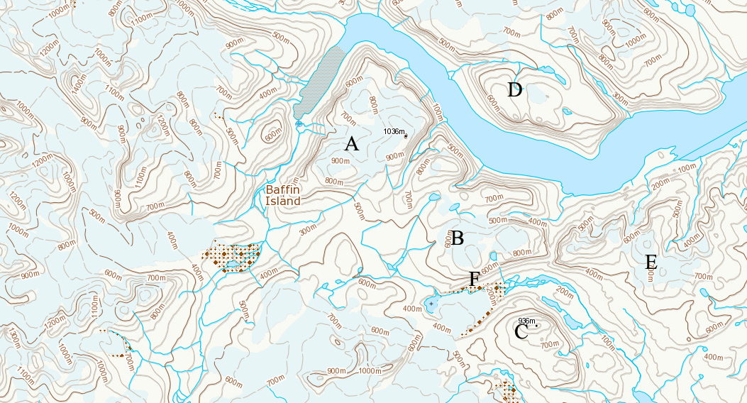
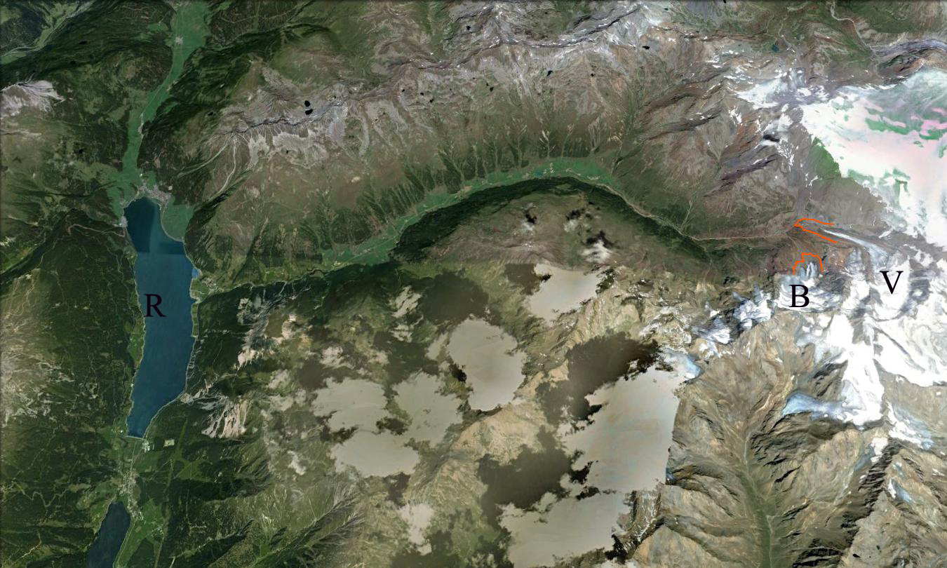
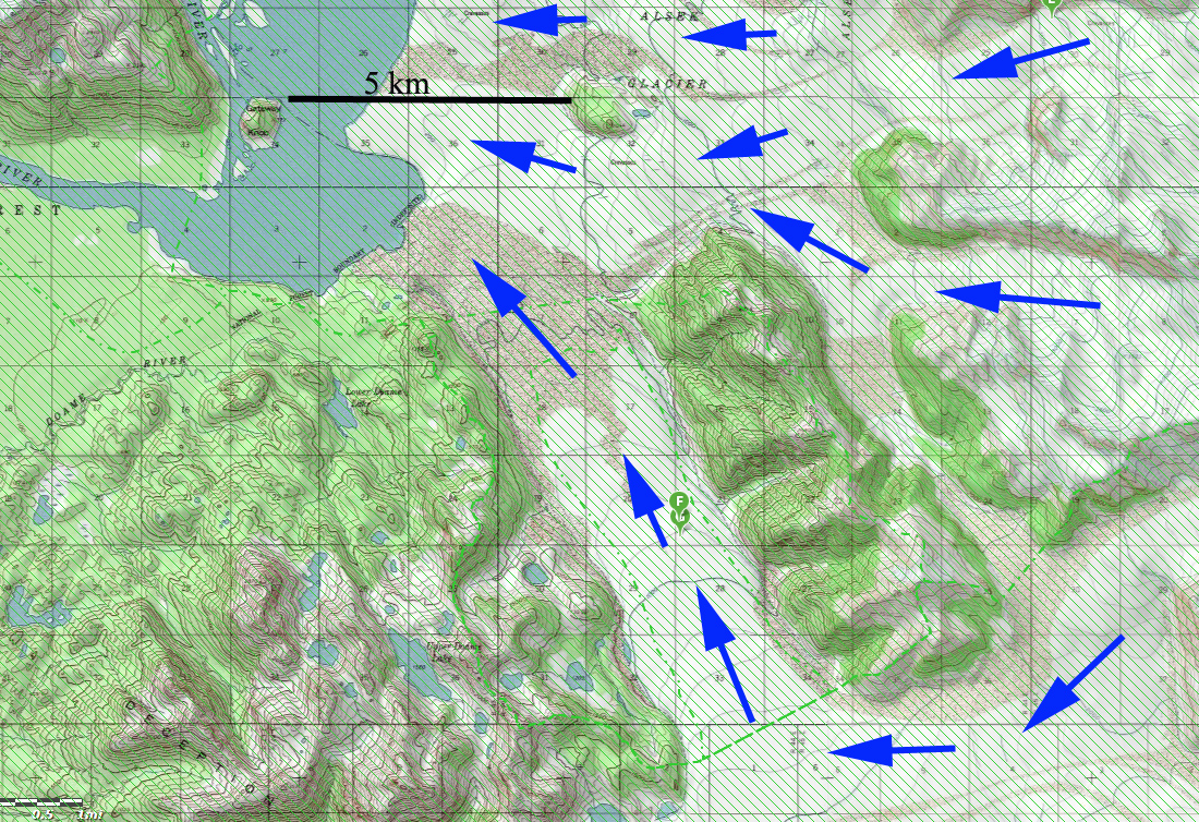
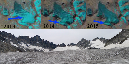
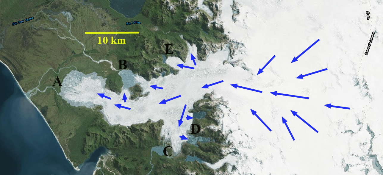
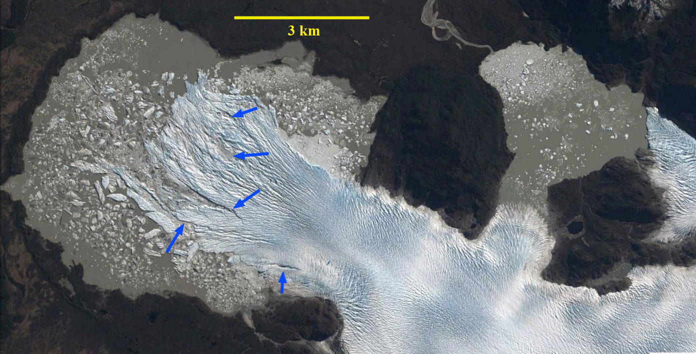
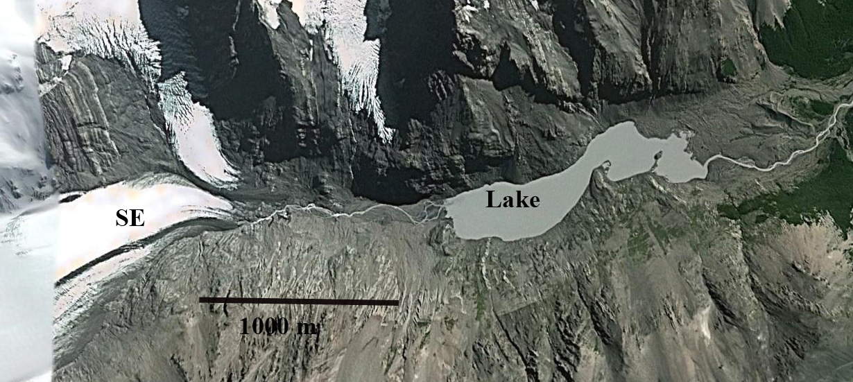
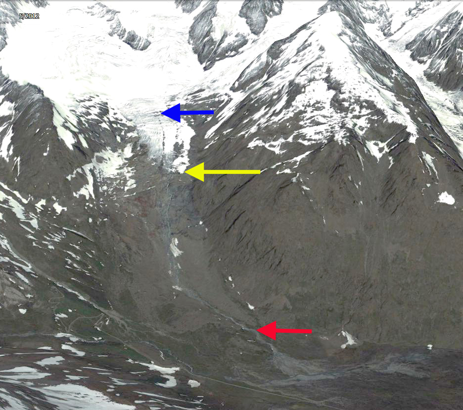
Google Earth image of Chubda Glacier. Blue arrows indicate flow, brown arrow indicates wide moraine dam, green arrow indicates shallow moraine areas.

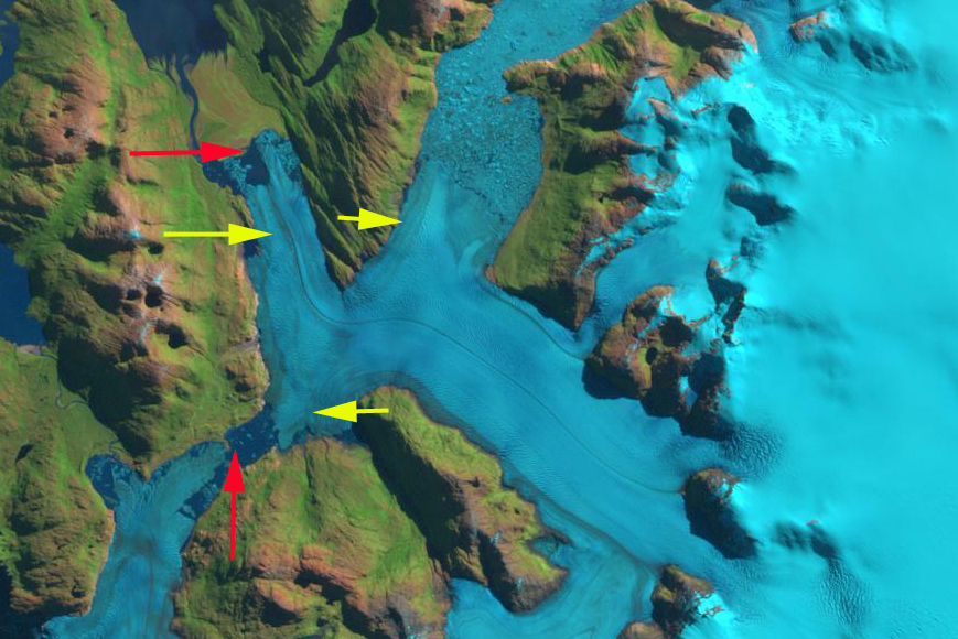
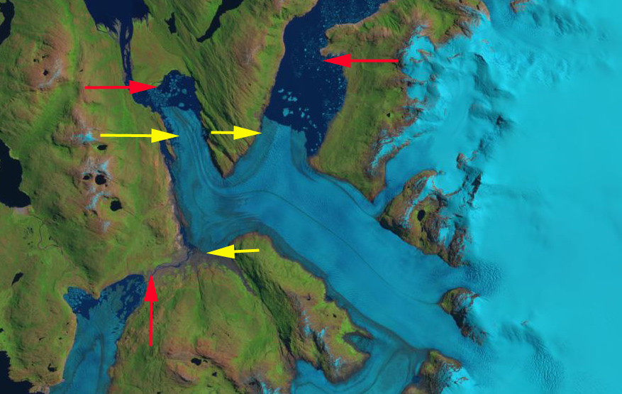
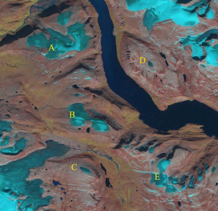
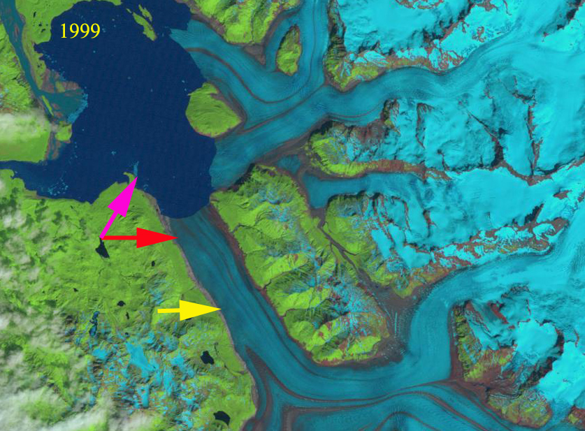
Chubda Glacier 2001 Landsat image. Red arrow indicates 1995 terminus location and yellow arrow is 2015 terminus location. Pink arrows indicate areas upglacier of expanding bedrock. Green arrow indicates moraine areas amidst the lake.

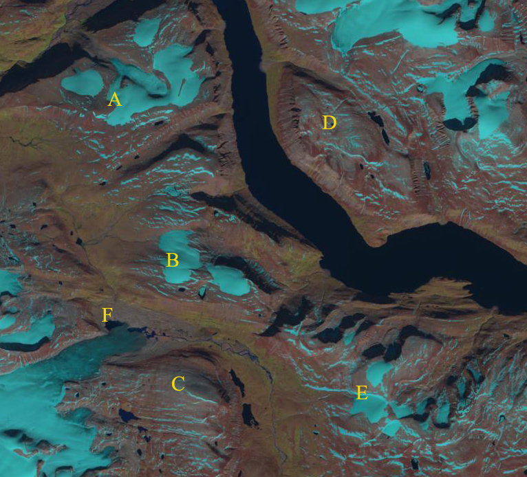
Chubda Glacier Landsat image in 2014. Red arrow indicates 1995 terminus location and yellow arrow is 2015 terminus location. Pink arrows indicate areas upglacier of expanding bedrock. Green arrow indicates moraine areas amidst the lake.