Mammoth Glacier, Wyoming Ongoing Retreat

On February 23, 2016May 2, 2024 By mspeltoIn climate change glacier retreat, glacier climate change, Glacier Observations

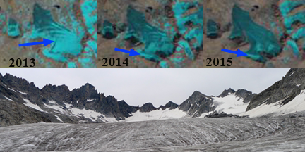
At top Landsat images from September 2013, 2014 and 2015 of Mammoth Glacier. The blue arrow indicates retained snowcover. A 2013 images of Mammoth Glacier from Sarah Meiser, note low slope and lack of crevassing above

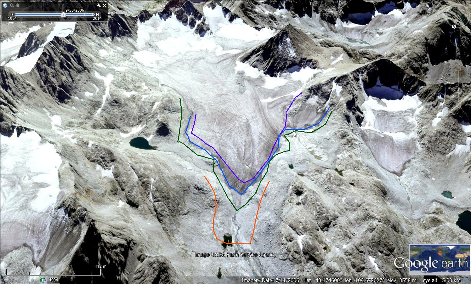
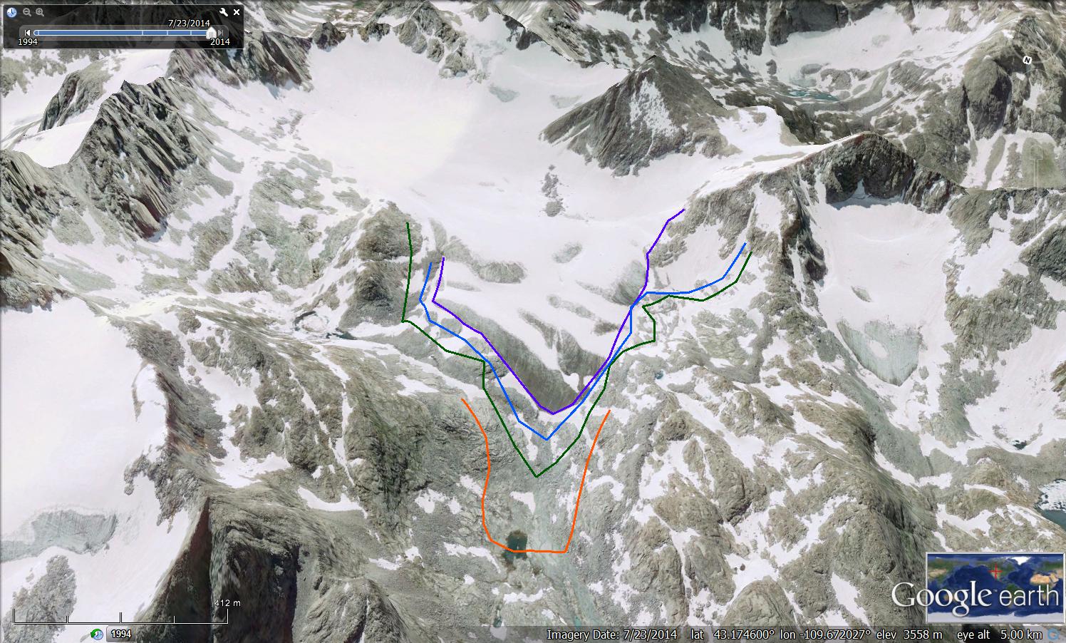
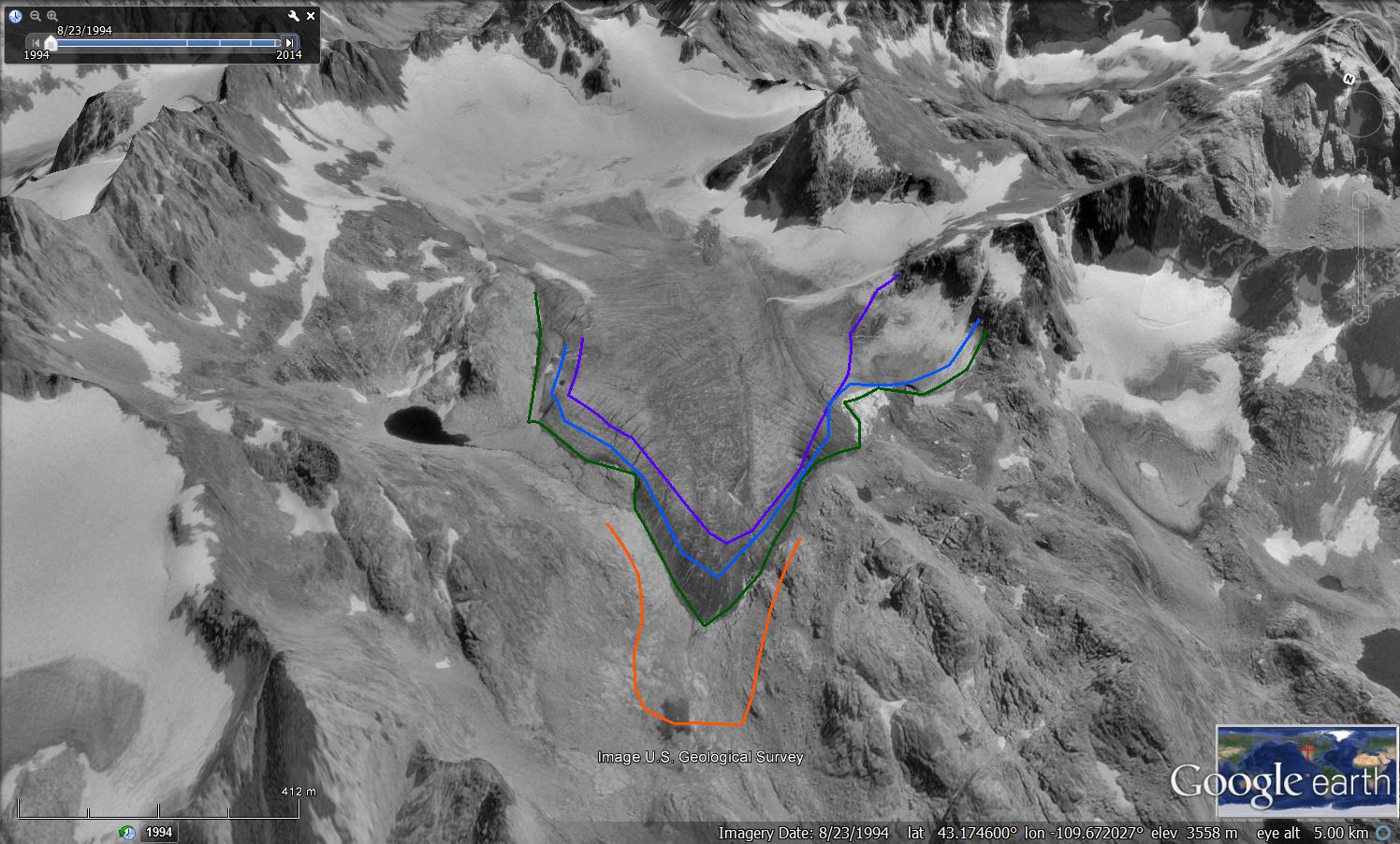
Mammoth Glacier is in the Wind River Range of Wyoming. The ongoing retreat is leading to a glacier that does not warrant the name mammoth for size, but soon it will for obsolescence.The long and low sloped glacier is the largest west of the Continental Divide in the range. The glacier is at the headwaters of the Green River and Green River Lakes. The glacier had an area of 4 square kilometers in 1952, 2.1 square kilometers in 2007 and 1.8 square kilometers in 2015. The Landsat sequence above from 2013, 2014 and 2015 illustrates the problem, insufficient retained snowcover to approach equilibrium, that is also evident in 2006 shown below. The setting is better illustrated with images from Sarah Meiser who I think has the best collection of recent images of Wind River Glaciers. A glacier like Mammoth with limited avalanching needs more than 50% retained snowcover at the end of the summer (accumulation area ratio) to be in equilibrium. In 2013 with three weeks left in the melt season, the accumulation area ratio (AAR) is slightly below 50%, note Sarah Meisel image below. In 2014 the AAR is 25 % and in 2015 the AAR is 5-8%. These periods of sustained bare ice exposure lead to area loss and thinning. A comparison of Google Earth images illustrate the area loss. In each image the orange line is the 1966 map position, green line 1994 margin, blue line 2006 margin and purple line 2014 margin. The loss in area at the margin is evident as is the loss on the western side between 2006 and 2014. Retreat has been 200 m from 1966 to 1994, 95 m from 1994-2006 and 95 m from 2006 to 2014. Area loss after the poor snowcover in 2015 will continue and the glacier will not long be considered mammoth in size. Pelto (2010) examined glaciers in the Wind River Range and found two-thirds could not survive current climate as they did not have a persistent accumulation zone, including Mammoth Glacier and Sacagawea Glacier. Thompson et al (2011) noted a 38% loss in area of the 44 Wind River Range glaciers from 1966-2006. Maloof et al (2014) noted an even larger drop in volume of 63% of the same glaciers from 1966-2012.

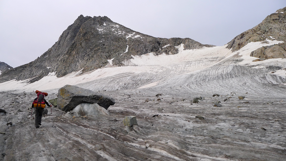
Sarah Meiser image illustrating how close to the top of the glacier the bare ice extends. This fact indicates that all of the firn had been lost, thus the area shown has not been a recent accumulation area.

1994 Google Earth Image

2006 Google Earth Image

2014 Google Earth image

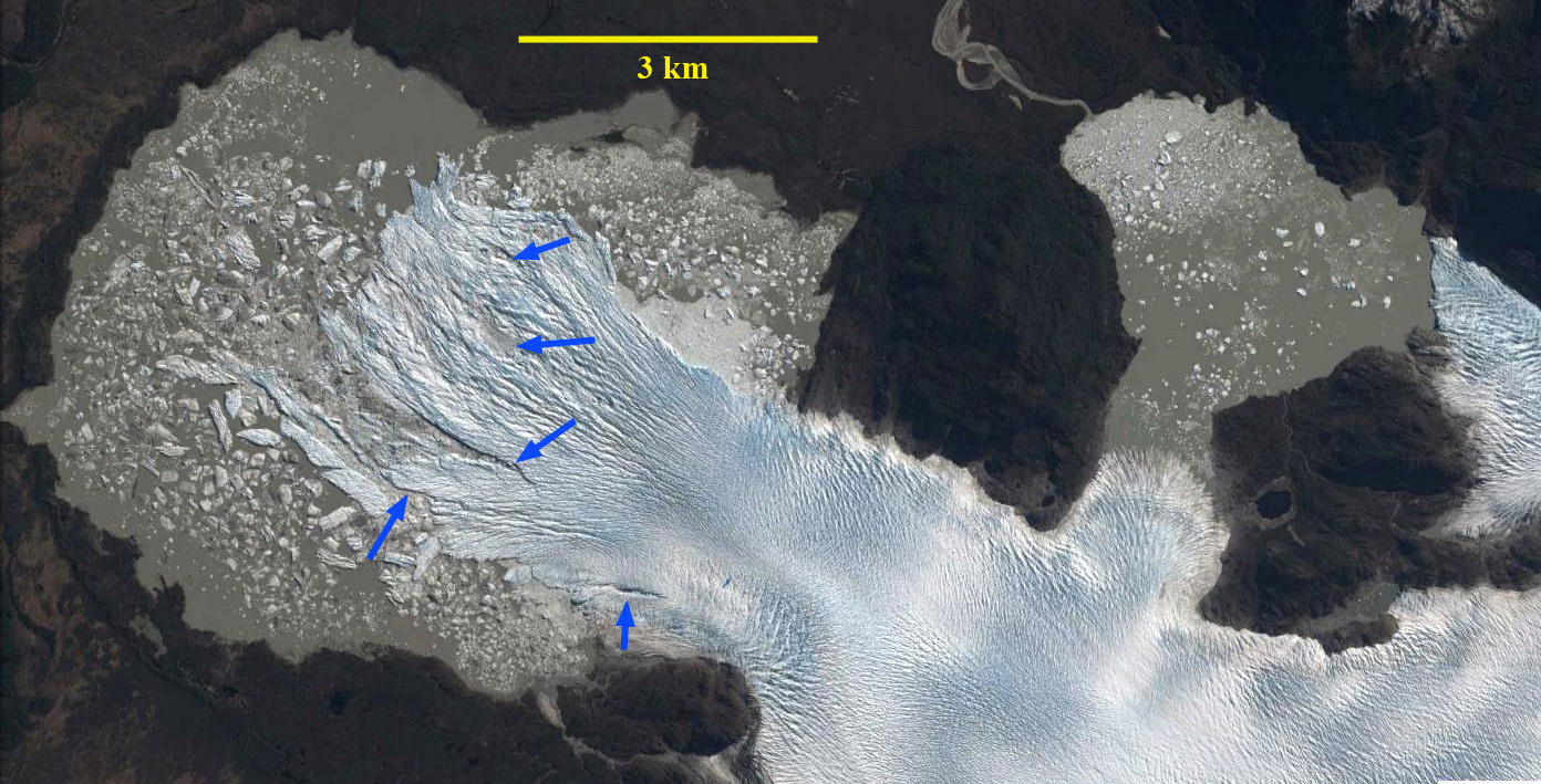
San Quintin Glacier, Chile terminus disintegration 1987-2015

On February 15, 2016May 2, 2024 By mspeltoIn chile glacier melt, chile glacier retreat, climate change glacier retreat2 Comments

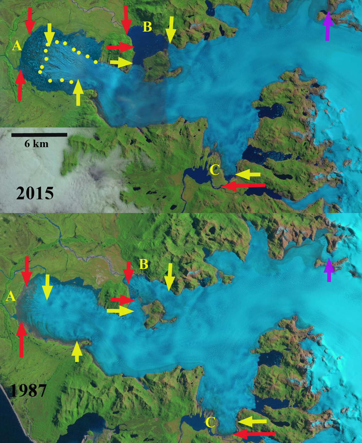
Landsat comparison of San Quintin Glacier in 1987 and 2015: red arrow indicates 1987 terminus location, yellow arrow indicates 2015 terminus location of the three main termini, and the purple arrow indicates upglacier thinning.

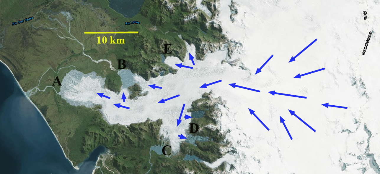
San Quintin is the largest glacier of the NPI at 790 km² in 2001 (Rivera et al, 2007). The glacier extends 50 km from the ice divide in the center of the ice cap. The peak velocity is 1100 m/year near the ELA (Rivera et al 2007), declining below 350 m/year in the terminus region. The velocity at the terminus has increased from 1987 to 2014 as the glacier has retreated into the proglacial lake (Mouginot and Rignot, 2015). The high velocity zone extends more than 40 km inland an even greater distance than at San Rafael (Mouginot and Rignot, 2015). Thinning rates in the ablation zone of the glacier are 2.3 m/year (Willis et al, 2012). The glacier has a low slope rising 700 m in the first 22 km. The low slope, broad piedmont lobe and many distributary terminus lobes is like the Brady Glacier, Alaska.

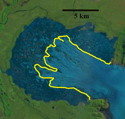
Davies and Glasser (2012) note that San Quintin Glacier terminated largely on land until 1991. The glacier has lost 15 % of its area in the last century (Davies and Glasser, 2012). The glacier has a main terminus and many subsidiary termini. In 1987 it is a piedmont lobe with evident minimal marginal proglacial lake development beginning. There is limited lake development at the main southern and northern terminus Point C and B respectively. Harrison et al (2001) observed that in 1993 the glacier terminus was advancing strongly into vegetated ground, while from 1996 to May 2000 the glacier underwent a transition between advance and retreat. The high rates of thinning are leading to the retreat not just of main terminus but the distributary terminus areas extending north and south into lake basins from the main glacier. From 1987 to 2015 the main terminus retreated 2200 m, almost all after 2000, largely through a disintegration of the terminus tongue in a proglacial lake. Extensive rifting of the terminus lobe in 2013 and 2015 is still apparent in imagery below, indicating this rapid area loss is not finished. The main lake, Point A, had an area of 23.8 square kilometers in 2011 (Loriaux and Cassasa, 2013) . The lake at Point B developing on the north side of the glacier, due to a 3500 m retreat, is now over 8 square kilometers. The southern terminus at Point C, has a narrow fringing lake and a retreat of 1100 meters from 1987-2015. The retreat here follows the pattern of Fraenkel Glacier, Acodado Glacier and Steffen Glacier to the south.

Digital Globe image of San Quintin Glacier in 2011.

2013 Google Earth image, with the large rifts indicating glacier weakness noted with blue arrows.

2015 Landsat image, yellow line indicates terminus. Note the tongue is surrounded on three sides by water.

Sierra de Sangra Glacier Retreat, Argentina

On February 9, 2016May 2, 2024 By mspeltoIn argentina glacier retreat, climate change glacier retreat, glacier climate change, Glacier Observations2 Comments

Comparison of four outlet glaciers of Sierra de Sangra in Argentina in a 1985 and 2015 Landsat image. Read arrow is the 1986 terminus location when all terminated in a lake. By 2015 only one terminates in a lake, yellow arrows.

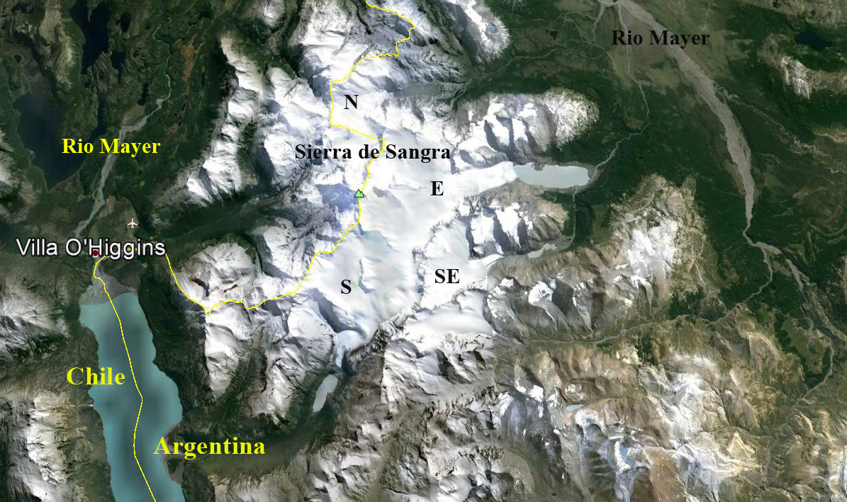
The Sierra de Sangra Range is located along the Chile-Argentina boundary with the east draining glaciers flowing into the Rio Mayer and then into Lake O’Higgins at Villa O’Higgins. Here we examine four glaciers that in 1986 all ended in lakes and by 2015 only one still terminates in the lake. Davies and Glasser (2012) noted the fastest retreat rate of this icefield during the 1870-2011 period has been from 2001-2011. NASA’s Earth Observatory posted an article on this blog post with better resolution images.

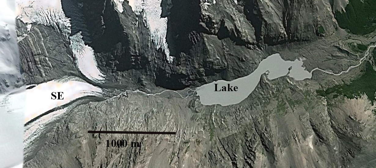
Sierra de Sangra is just east of Villa O’Higgins with the crest of the range on the Chile Argentina border. The four glaciers examined here are indicated by S, SE, E and N.

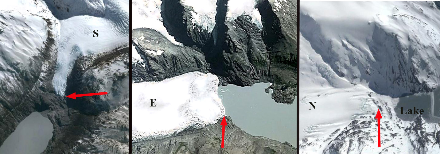
The South Outlet Galcier (S) has retreated 700 m from 1986 to 2015 and terminated in a lake in 1986. By 2015 it terminates on a steep slope well above the lake. The Southeast Outlet Glacier (SE) terminates in a lake in 1986. By 2015 it has retreated 1200 m to a junction with a tributary from the north. The East Outlet Glacier is the largest glacier and has retreated just 300 m from 1986 to 2015. There is a sharp elevation rise 200 m behind the terminus, which likely marks the end of the lake basin. This is marked by a crevasse zone. The North Outlet Glacier (N) ended in a lake in 1986. By 2015 it has retreated 700 m and ends on a bedrock slope well above the former lake level. All of the glaciers have an accumulation zone in each satellite image examined. This indicates they can survive present climate. The glacier retreat is not as large as Cortaderal Glacier and Glaciar Del Humo.

Google Earth images from 2013 of the terminus of three outlet glaciers above and one below. The red arrow indicates terminus location. Three of the four no longer terminate in a lake.

Orpissuup Tasia Glacier slowdown, SW Greenland

On December 30, 2015May 2, 2024 By mspeltoIn climate change glacier retreat, glacier climate change, Greenland glacier retreat

Tedstone et al (2015) Figure 3 illustrates the widespread velocity decline along three transects.

Pelto et al (1989) after a field campaign we mounted in 1985 and 1986 on Jakobshavns Glacier noted that the velocity was essentially the same in the summer of 1964, 1976, 1978, 1985 and 1986. Further we observed that the agreement between surface mass-balance and volume-flux calculations, suggested that “Jakobshavns Isbrae: is almost in a state of equilibrium”. The point of the study was to establish a baseline of velocity before the anticipated acceleration due to warming. This acceleration due to warming happened beginning in 1992 from 20 m/day at the calving front in 1985 to 46 m/day in 2012, comparing the same locations the annual speed increase was 282% from 1992 to 2012 (Joughin et al 2014). The Jakobshavns Isbrae is a tidewater glacier, just south of the glacier the margin of the ice sheet is dominated by a land terminating section that has a different dynamic response to warming.

Tedstone et al (2015) in a paper published in Nature in October noted a decadal reduction in glacier velocity for a land terminating region of the Greenland Ice Sheet. This slow down occurred despite a 50% increase in meltwater production. This is emphasized in the figure above indicating the changes along three transects from green earlier to purple later years. A glacier inhabits a particular topographic environment that establishes the basic flow field. Climate change can affect glacier flow by increasing ice melt, which leads to ice thinning and a consequent reduction in force generating ice deformation and flow. This same ice melt can deliver meltwater to the base of the ice sheet, which can lead to short term increases in basal water pressure that will drive acceleration, the acceleration tends to be short lived. The overall impact of these competing forces is what this study indicates, that just as is the case on alpine glaciers thinning resulting from more melt leads to velocity reductions as a more efficient hydrologic system develops reducing basal water pressure. This same process clearly does not apply to calving tidewater outlet glaciers. Here we examine the changes at the terminus, evidence of thinning and location of moulins on the outlet glacier that flows into a series of lakes, Orpuussit Tasia, along Transect B.

Landsat image comparison from 2000 and 2015.

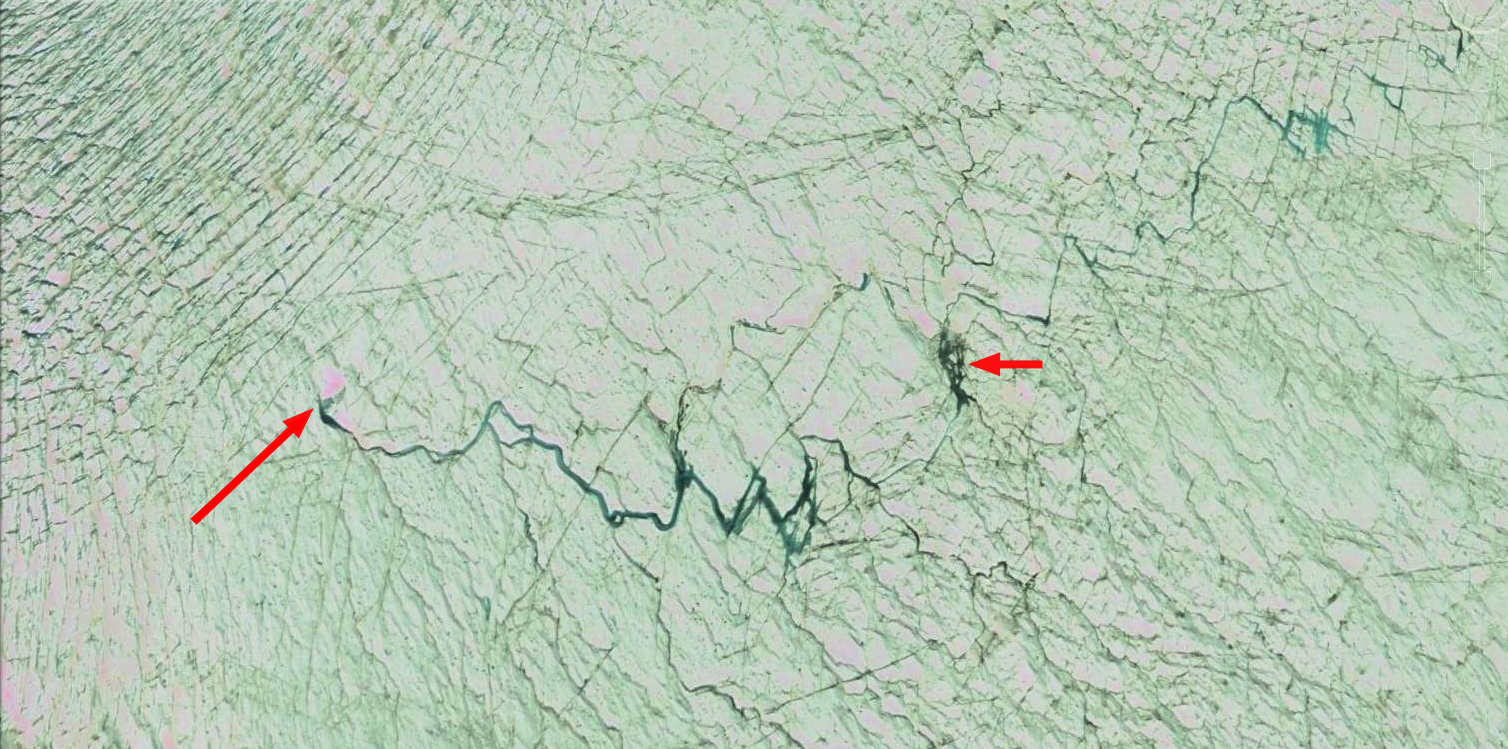
In the comparison of Landsat images above from 2000 and 2015 the expansion of small proglacial lakes is evident at each red arrow, #2 has the greatest expansion. At the yellow arrows thinning is evident at a small lake that is fed by glacier runoff giving it a green sediment laden color, and by 2015 no longer receives meltwater as the ice sheet has thinned below the watershed divide, yielding clearer water which appears darker. The expansion of the end of the medial moraine also indicates thinning. Four bedrock areas emerging from the ice have much greater prominence in 2015 than 2000 purple arrows. This is modest thinning and retreat compared to the Jakobshavn and other large outlet glaciers to the north. The first image below indicates the terminus with red dots in a Google Earth image. The terminus as the proglacial lake #2 is pinned on a two bedrock prominences which should slow retreat. Proglacial lake #3 does not have an evident pinning point, and should retreat back towards the peninsula to the south in the near future. The second image below indicates the supraglacial streams and moulins in a small area of this glacier. The linear nature of many streams indicate they are occupying former crevasse features. Just as in the 1980’s little of the runoff reaches the terminus at the surface, almost all is directed to the base via moulins. Tedstone et al (2015) found that velocity did increase in summer, but declined more in the winter. NASA Landsat and Nasa Earth Observatory provides several excellent figures and explanation of the process in the study area.

Google Earth image indicating ice sheet margin in 2012, red dots.

Google Earth image indicating surface streams and locations of two moulins.

Lex Blanche Glacier Recession, Mont Blanc Massif, Italy

On December 28, 2015May 2, 2024 By mspeltoIn climate change glacier retreat, Glacier Observations, Italy glacier retreat

Lex Blanche Glacier (Lb) comparison in a 1990 and 2015 Landsat image. Red arrow indicates 1990 terminus, yellow arrow the 2015 terminus and the purple arrow a separated tributary. Debris covered Miage Glacier (M) is adjacent.

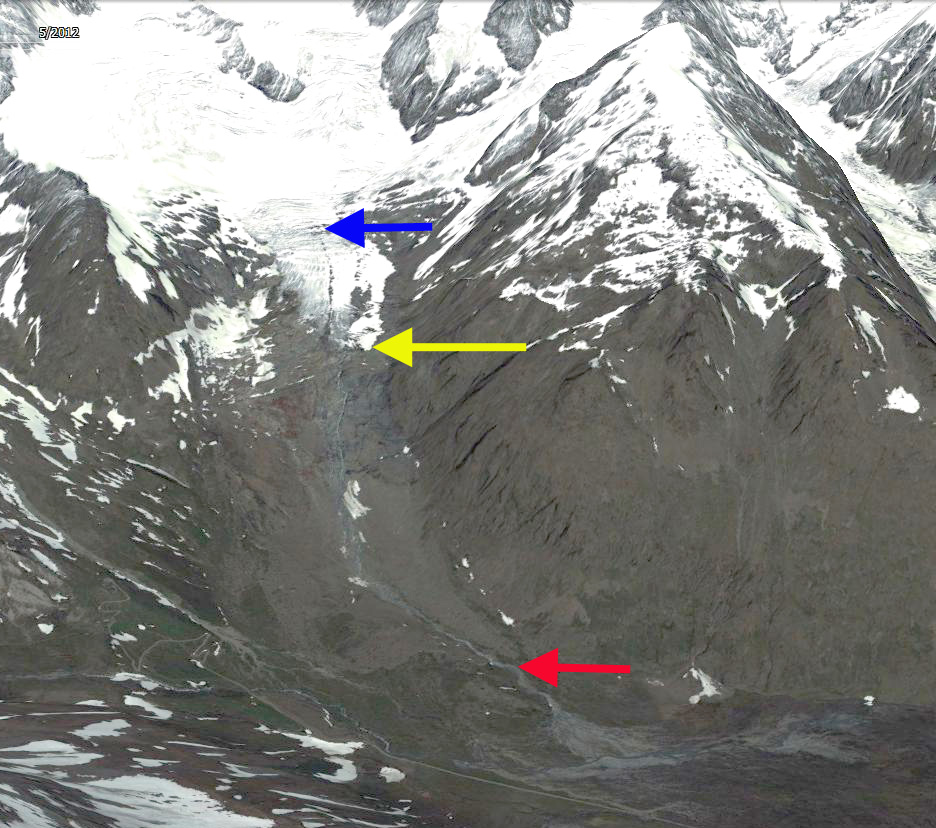
Lex Blanche Glacier descends from 3500 m on the southeast flank the Aiguille de Glaciers of the Mont Blanc Massif into the Vale Veny of Italy. The glacier is adjacent to Miage Glacier (M). The glacier advanced over 700 m from 1970 to 1990. In 1990 the glacier extended to the base of a steep slope and turned north to terminate at 1980 m. By 2001 the glacier has retreated up a steep slope to near where the 1970’s advance had begun. By 2009 and 2011 further retreat has left the terminus just above a particularly steep bedrock slope. By 2015 the glacier has retreated 1100 m and terminates at 2450 m remaining on a relatively steep slope. The glacier is heavily crevassed a short distance above the terminus suggesting the period of rapid retreat should be ending. A tributary from the north has detached from the main glacier at the purple arrow. In recent warm summers the glacier has retained snowcover above 3150 m. The mass balance noted in Figure 8 (see below) of a paper by Berthier et al (2014) indicates the thinning is glacier wide but most prominent on glacier tongue. Berthier et al (2014) used the Pléiades satellites to identify a negative region wide mass balances of glaciers in the Mont-Blanc area of -1.04 m/year for the 2003-2012 period. The meltwater runoff from this glacier feeds the Dora Baltea River and then the Po River. Both rivers feature extensive hydropower including the Champagne and Nus hydropower plant on the Dora Baltea that produce 41 MW. The retreat of this glacier mirrors that of other glaciers of Mont Blanc including Taconnaz, Bionnassay, Mer de Glace and Tour Glacier.

Figure 8 from Berthier et al (2014) on glacier wide mass change with thinning in browns, and darker browns greater thinning.

Google Earth image from 2001 indicating the 1990 terminus at red arrow and 2001 terminus at yellow arrow.

Google Earth image from 2009 indicating the 1990 terminus at red arrow and 2009 terminus at yellow arrow.

Google Earth image from 2011 indicating the 1990 terminus at red arrow and 2011 terminus at yellow arrow. Blue arrow indicates the lowest heavily crevassed region.

Kanchenjunga Glacier, Nepal Volume Losses

On December 23, 2015May 2, 2024 By mspeltoIn climate change glacier retreat, glacier climate change, Himalaya glacier retreat2 Comments

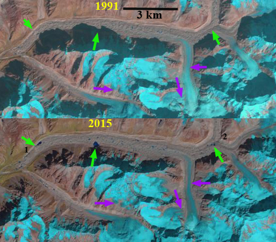
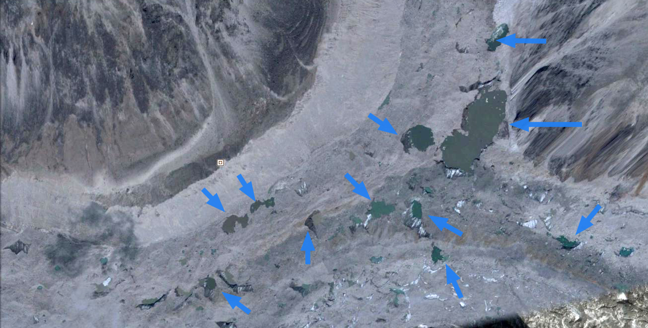
Figure 10-16. Kanchenjunga Glacier (K) from 1991 to 2015, green arrows indicate locations of enhanced supraglacial lakes since 1991. Purple arrow indicates areas of thinning at higher elevations in the region. Location 2 is the main junction area.

Kanchenjunga Glacier is the main glacier draining west from Kanchenjunga Peak, also listed on maps as Kumbukarni. The glacier is similar to Zemu Glacier flowing east from the same mountain into Sikkim, in the heavy debris cover that dominates the glacier in the ablation zone extending from the terminus for 15 km and an altitude of 5600 m. Identifying the retreat is difficult due to the debris cover. Racoviteanu et al (2015) examined glaciers in this region using 1962 and 2000 imagery. They found area losses of 14% for debris covered glacier and 34% for clean glaciers. The debris covered glaciers terminus response is even more muted indicating why terminus change is an easy measure of glacier change but not always the best. For Kanchenjunga Glacier Racoviteanu et al (2015) indicate the glacier area declined by just 4-8% from 1962-2000.

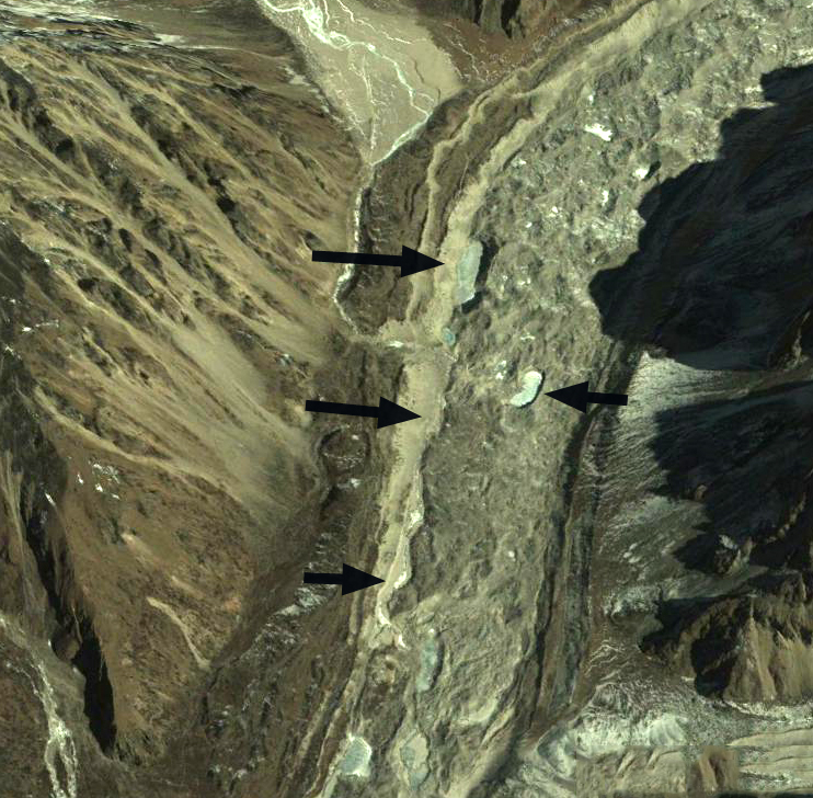
What is apparent in the Landsat images at the green arrows is the increase from 1991 to 2015 of supraglacial lakes. Also features of thinning are evident in the mid reaches of the glacier, purple arrows, where tributaries have narrowed and detached from the main glacier. A closeup of the main glacier junction 12 km above the terminus indicates the number of large supraglacial lakes. These cannot form in a region where melting does not dominate over glacier motion. The Google Earth image from 2014 of the terminus area indicates a patchwork of moraine cored ice dotted with supraglacial lakes and dissected by the glacial outlet river in the lower 3 km of the glacier. This is clearly not an active portion of the glacier, it is thin not moving and does not fill even the valley floor. An overlay of images indicates the lack of motion. The heavy debris cover has slowed retreat and thinning, however, the lower glacier is poised for an increased rate of retreat with merging of supraglacial lakes, which will lead to further area losses. The Kanchenjunga Glacier is losing volume like all other 41 glaciers examined in detail and linked at the Himalayan Glacier Index page.

Google Earth image of the main glacier junction region (2) Supraglacial lakes in the area of at 5200 m.

Google Earth image of supraglacial lakes 2-5 km above the terminus and the region along the north margin of the glacier where the glacier is receding from the lateral moraine.

2014 Google Earth image of terminus reach. Black arrows indicate ice cored moraine, blue arrow the lowest large supraglacial lake, 2.5 km above the terminus and red arrow the last remnant of ice.

Dawes Glacier, Alaska Retreat and Harbor Seals

On December 17, 2015May 2, 2024 By mspeltoIn climate change glacier retreat, glacier climate change, Glacier Observations

Comparison of 1987 and 2015 Landsat images of Dawes Glacier. Red arrow 1987 terminus, yellow arrow 2015 terminus, pink arrow location where tributaries separated.

Dawes Glacier terminates at the head of Endicott Arm, a 55 km long fjord in southeast Alaska. Dawes is a major outlet glacier of the Stikine Icefield. Larsen et al (2007) observed a rapid thinning of the Stikine Icefield and that Dawes was thinning faster than all but Muir Glacier in Southeast Alaska during the 1948-2000 period. During the period from 1891 when first mapped and 1967 the glacier retreated 6.8 km (Molnia,2008). The retreat has been driven by rising snowlines in the region that has driven the retreat of North Dawes, Baird and Sawyer Glacier.

A comparison of 1987 and 2015 Landsat images illustrate recent retreat and thinning of the glacier. The main terminus retreated 1100 m during this interval, a reduced rate from the previous period from 1978 to 1987 the glacier retreated 2.8 km. Key tributaries at the purple and green arrow each have a 30% decline in width. At the pink arrows are three tributaries that fed the Dawes Glacier in 1987 and are now detached. This fragmentation will continue. The reduced inflow and up glacier thinning is ongoing as will the retreat. A key mechanism for retreat over the last century has been calving. The calving rate has declined of late, possibly due to reduced water depth. The 2007 Hydrographic map of the area indicates water depth at the calving front still over 100 m., with a depth of 150 m 1 km down fjord of the terminus (see bottom image). Examination of surface elevation portrayed in Google Earth indicate a relatively sharp rise near the first junction, the surface elevation being at 1400 feet. The trimline is noted with blue arrows, note how much higher above the ice the tramline is at the terminus than at 1400 feet. At this point the northern arm would appear to have a bed above sea level and the main arm at least a much shallower bed. Pelto and Warren (1991) observed the calving rate reduction with water depth in the area. Note the ogives, curved bands, on the northern arm that form once per year at the base of icefall due to seasonal velocity change. The glacier thinning is continuing, but the retreat rate will decline as the fjord head is approached. As calving is reduced harbor seals will be disappointed as they like us are drawn to glaciers.

Google Earth image of Dawes Glacier in 2013. Blue arrows indicate trillion and number are elevation in feet.

The Alaska Department of Fish and Game has been monitoring harbor seals in the fjord and noting their use of icebergs and proximal glacier regions. The noted that females travel to pup on the icebergs in the spring and also utilize the are for mating. Because there was little information on where seals that use glacial habitat during pupping and mating season spend the remainder of the year, ADFG attached satellite tags to harbor seals to monitor their movements. In 2008 this data indicated that that adult and sub-adult seals captured in Endicott Arm early summer spent the late summer and fall months in Stephens Passage, Frederick Sound, Chatham Strait, This study is in part prompted by a decline of harbor seals in the Glacier Bay region where they also utilize icebergs, as NPS biologist Jamie Womble explained at the AGU 2015 meetin

1978 Landsat image, blue arrow 1978 terminus, red arrow 1987 terminus and 2015 terminus yellow arrow. Note the improvement in the Landsat imagery.

Emmons Glacier, Washington Velocity Map Signals its Future

On December 14, 2015May 2, 2024 By mspeltoIn climate change glacier retreat, glacier climate change, Glacier Observations1 Comment

1966 Aerial image taken by Austin Post, USGS, red arrow indicates discharge stream. Emmons Glacier in 2005, red arrow indicates discharge stream, blue arrow lower limit of clean ice and green arrow region of peak velocity.

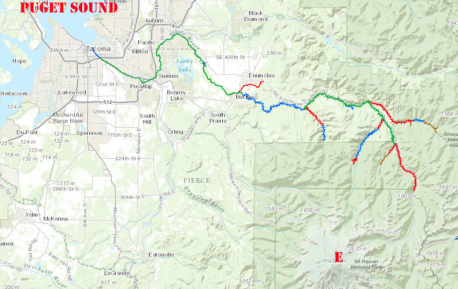
Emmons Glacier descends the northeast side of Mount Rainier into the White River, and is its largest glacier by area The river is host to pink, chum, coho and chinook salmon, note distribution map below. The lower glacier is heavily debris covered from a landslide off of Little Tahoma in 1963, the glacier was advancing at the time and continued to advance into the early 1980’s , maintaining the advanced position until 1994. Retreat was negligible from 1994-2003. Since 2003 retreat has increased but is still modest. Thinning of the ablation zone has been ongoing and has been more significant than retreat. The National Park Service mass balance work led by Jon Riedel indicates an approximate 10 m thinning from 2003-2014.

White River chinook salmon distribution from the Washington Department of Fish and Wildlife SalmonScape, green=rearing, red= documented spawning blue=documented presence.

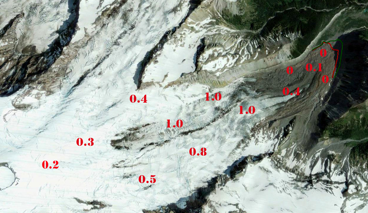
A recent paper by Allstadt et al (2015) examines velocity on this glacier using terrestrial radar interferometry. There key observations are that: Emmons has a slow velocity near the summit < 0.2 m per day , high velocities over the upper and central regions 1.0–1.5 m per day and stagnant debris-covered regions near the terminus < 0.05 m per day. That glacier movement is mostly via sliding. Lastly that there is a large seasonal decrease from July to November. The late summer slowdown is typical of alpine glaciers, where despite peak melt, the drainage system is well developed and basal water pressure is reduced as a result.

The image below indicates velocity distribution in a cursory fashion compared to the excellent detail of Allstadt et al (2015). The glacier has had a negative mass balance in recent years and this combined with the lack of glacier movement near the terminus, indicates this section of the glacier will continue to melt away, slowed by the insulating debris cover. Google Earth images from 1994 and 2012 indicate an approximately 200 m retreat in the glacier center, and evident thinning in the region up to the yellow arrows. In 2015 record melt was observed in the North Cascades and at least through mid-summer on Mount Rainier. Currently the area of the glacier has not decline enough to reduce late summer streamflow which would impact salmon during the low flow period.

Velocities noted by Allstadt et al (2015) displayed on Google Earth image.

1994 Google Earth Image, red is 2012 terminus position, green the 1994 terminus position

2012 Google Earth Image, red is 2012 terminus position, green the 1994 terminus position

Twin Glacier, Alaska Retreats from Twin Lake

On December 3, 2015May 2, 2024 By mspeltoIn alaska glacier retreat, climate change glacier retreat, glacier climate change, Glacier Observations1 Comment

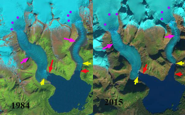
Landsat image comparospm pf 1984 and 2015. The yellow arrow indicates 2015 terminus, red arrow the 1984 terminus, pink arrows the ogives and purple dots the snowline on the day of the image.

Twin Glacier is an outlet glacier of the Juneau Icefield flowing south into the Taku River valley, terminating in Twin Lake. There are two terminus arms the East and West Twin Glacier are receding up separate fjords, though they are fed from a joint accumulation zone. The Juneau Icefield has been a focus of study by the Juneau Icefield Research Program since 1946. This program led to my first visit to the glacier as a member of the program in 1982 and again in 1984. Both glacier arms have pronounced ogives formed in the icefall that descends from the accumulation zone into the valley reach ablation zone. Ogives form annually from the seasonal variation of velocity through the icefall. An examination of the change in Juneau Icefield glaciers using Landsat images from 1984 and 2013 identify a significant retreat that has continued into 2015.

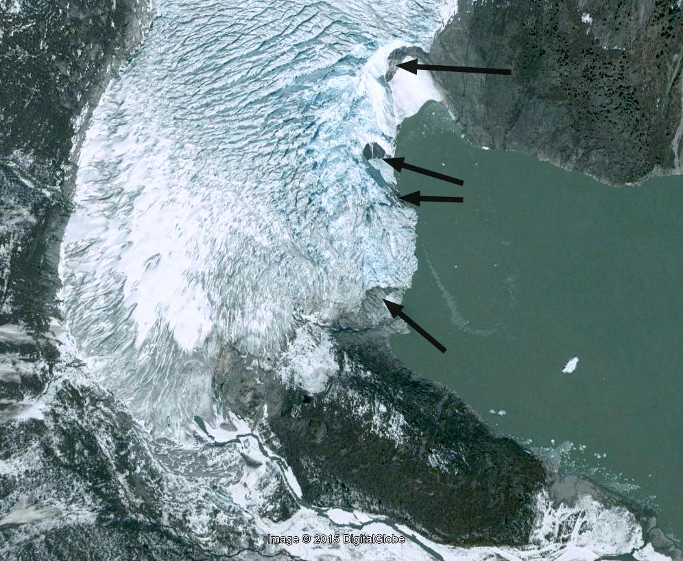
The West Twin has retreated 600 m from 1983 to 2013, at an elbow in the fjord. Elbows like this are often good pinning points that are a more stable setting. This elbow also represents the point at which the glacier terminus is pulling out of the lake that it is calved into for over a century. The bedrock at the terminus is evident in both 2006 imagery and a 2015 image from the Wings Airways five glacier seaplane discovery tour, black arrows. The glacier will no longer be calving, which should also slow the retreat rate.

Google Earth Image 2006

2015 Wings Airways image

The East Twin is the narrower glacier and drops more quickly in elevation. The glacier has retreated 900 m from 1984 to 2015. The terminus has calved into Twin Lake for over a century, but in 2015 the width of the terminus calving into the lake has declined to 150 m from 600 m in 1984. The bedrock exposed on either side of the terminus indicates the terminus is on the verge of retreating from the lake. The black arrows indicate both bedrock at the glacier front, but also the trimlines left from recent thinning. The Google Earth image from 2006 and the 2015 image from the Wings Airways five glacier seaplane discovery tour.

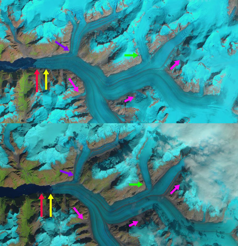
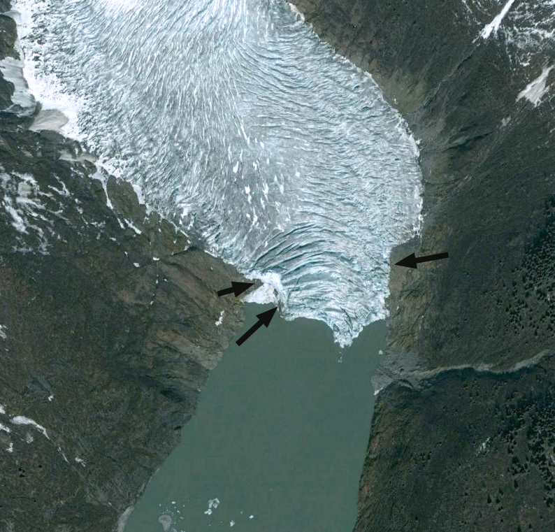
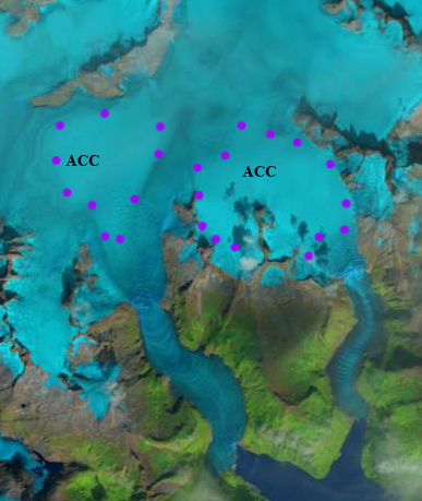
In 2015 the snowline was particularly high, the accumulation zone usually covers the entire reach of the broad high elevation accumulation zone, not the pockets indicated by the purple dots. The declining mass balance identified by the Juneau Icefield ongoing mass balance program, which the high snowlines is indicative of is what is driving the retreat (Pelto et al, 2013).

Google Earth Image

Wings Airways Image

August 2015 Landsat image of Twin Glacier. The purple dots outline the accumulation zone where snowpack was retrained from 2015.

A Voice for Glaciers at COP21

On November 27, 2015May 2, 2024 By mspeltoIn climate change glacier retreat, glacier climate change, Glacier Observations

During the last six years From a Glaciers Perspective has published 520 Posts examining the response of glaciers to climate change. No hyperbole has been needed to use words such as disappear, fragmented, disintegrated, and collapse. Glacier by glacier from the fragmentation of glaciers to the formation of new lakes and new islands has emphasized the changing map of our world as glaciers retreat. The story details change, but the story remains the same; glaciers are poorly suited for our warming climate, and their only response is to hastily retreat to a point of equilibrium, which many will not attain, and some have already ultimately failed. The Gallery below is a mere snippet of the changes that are occurring. These are illustrations of why our paper this year led by the World Glacier Monitoring Service team was titled Historically unprecedented global glacier decline in the early 21st century. As the UN Climate Change Conference 2015 in Paris, COP21 begins, since no glaciers are invited, there story must be told in pictures, data and our words.

Data: World Glacier Monitoring Service Mass Balance Time Series for Alpine Glaciers.

Pictures

Words:

After 34 consecutive summers working on glaciers, there is occasion to speak as more than just a scientist, since glaciers do not have a voice people hear.

Paierbreen Rapid Calving Retreat, Svalbard

On November 23, 2015May 2, 2024 By mspeltoIn climate change glacier retreat, glacier climate change, Glacier Observations, svalbard glacier retreat

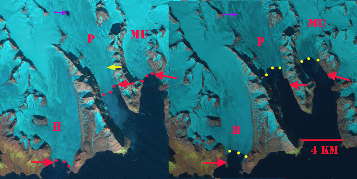
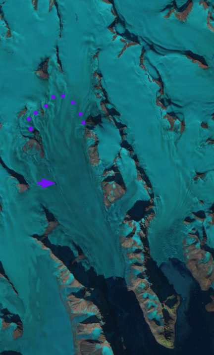
1990 and 2014 Landsat images indicating Paierbreen (P), Muhlbacherbreen (MU) and Hansbreen (H). The red arrow and red dots indicate the 1990 terminus location and yellow arrows and yellow dots the 2014 terminus location. The purple arrow indicates the location of a supraglacial lake that was persistent in the 1990’s but is no longer evident in 2013, 2014 and 2015.

From 1990 to 2014 all four of the glaciers terminating along the north coast of Hornsund have retreated significantly: Hansbreen (H), Paierbreen (P), Muhlbacherbreen (MU), Storbreen. Svalbard is host to 163 tidewater glaciers with a collective calving front of 860 km (Błaszczyk et al, 2009). Nuth et al (2013) determined that the glacier area over the entire archipelago has decreased by an average of 80 km²per year over the past 30 years, a 7% reduction. In the most recent period 1990-2007, terminus retreat was larger than in an earlier period from 1930-1990, while area shrinkage was smaller. Hornsund is a fjord that in 2014 almost cuts through the southern Island of Svalbard. The Institute of Geophysics Polish Academy has maintained a Polish Research Station in Hornsund since 1957. The 1984 map, from the University of Silesia, of the glaciers and geomorphology document the extent of the glaciers in 1983. A more detailed examination by the same researchers, Blaszczyk et al. (2013) reported the total area of the glacier cover lost in Hornsund Fjord area from 1899–2010 was approximately 172 square kilometers. This groups ongoing research, Petlicki et al (2015) , identified the impact of a waterline notch that enhances calving at Hansbreen. This study identifies the importance of water temperature and reduced sea ice cover in the fjord.

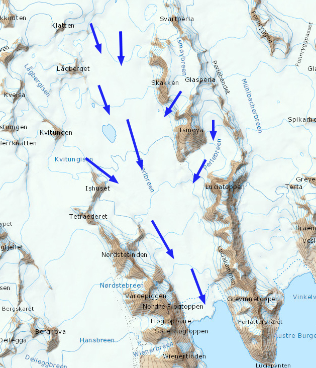
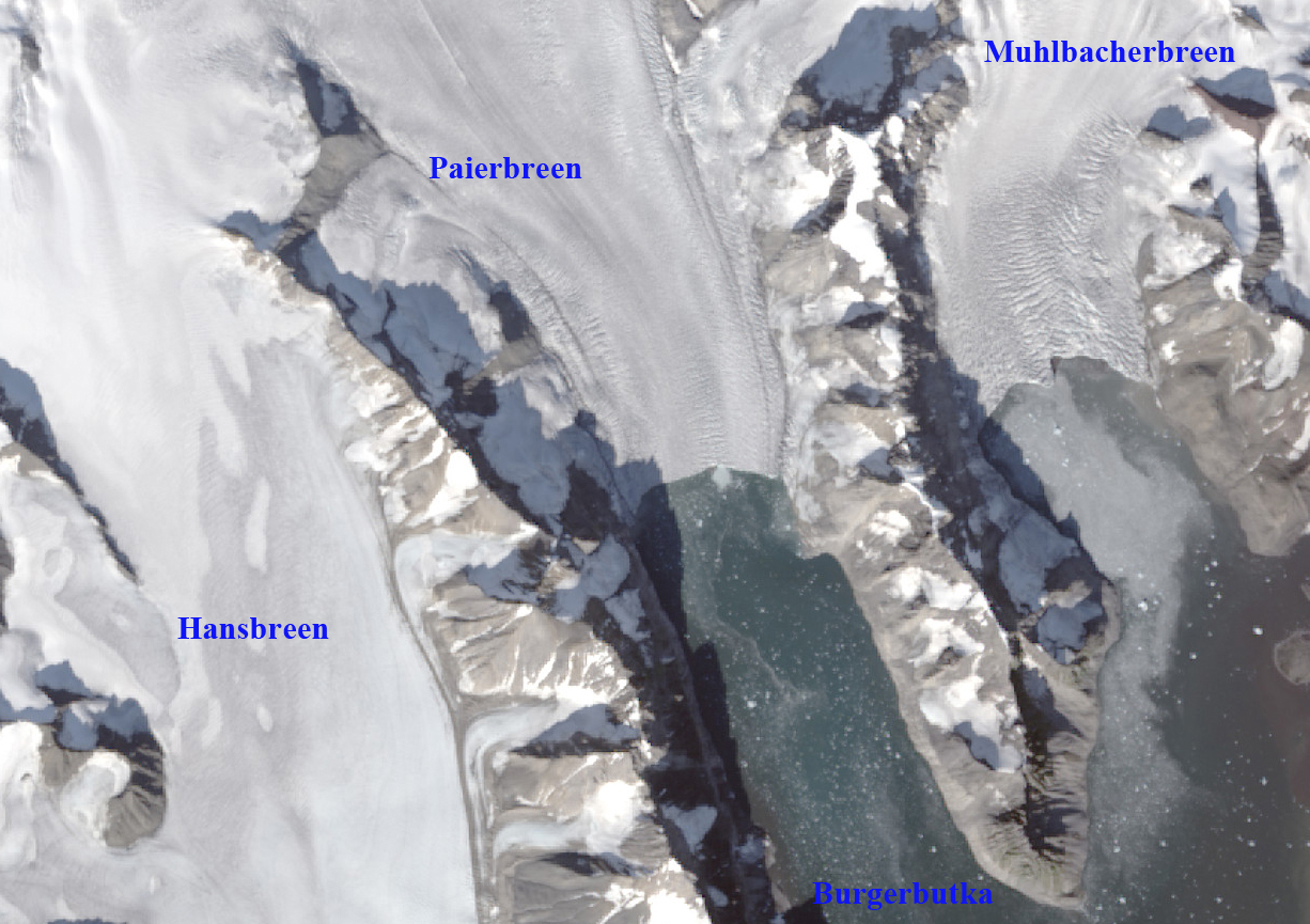
Paierbreen in 1990 terminated in Burgerbutka with a 1900 meter long calving front. At the purple arrow a supraglacial lake existed that is also seen in the TopoSvalbard Map. The snowline on Paierbreen is further upglacier of the calving front than for the adjacent glaciers indicating a lower surface slope. By 2014 the glacier has retreated 2200 m with the current terminus at a narrow point in the fjord. Beyond this point the fjord again expands, which will enhance calving and retreat. There is no significant step in glacier slope indicating where the tidewater limit is, given the low slope, it is not likely close to the current ice front. The calving front is 1600 m wide in 2014. The supraglacial lake is only a sliver in 2013 and 2014. The snowline in the Landsat image from 2013 is at 450 m. The story of retreat here is the same as at Samarinbreen and Hornbreen

2013 Landsat Image

Topographic Map from TopoSvalbard

Satellite Image from TopoSvalbard

Zhizhai Glacier Retreat, Lake Expansion, China

On October 29, 2015May 2, 2024 By mspeltoIn china glacier retreat, climate change glacier retreat

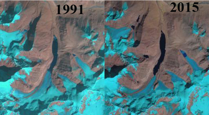
Fig. H. Zhizhai Glacier change from 1991 to 2015, red arrow indicates 1991 terminus, yellow arrow 2015 terminus and purple arrow indicates areas of thinning. Green arrow indicates another lake growing with glacier retreat.

Located between Longbashaba Glacier and Jimi Glacier, this glacier extends 4.75 km north from the Nepal-China border in the southeast region of the Pumqu River basin. The moraine dammed glacier lake, Zhuxico Lake, poses some risk to the 23 villages downstream of the lake and the Rongkong Hydropower station. This risk has been examined for another lake in the basin Longashaba by Yao et al (2012). Che et al (2014) report on an inventory of glaciers and glacier lakes in the Pumqu Basin, and note that lake expansion is higher from 2001-2013 than for the 1970-2000 period, posing greater threats for a glacier lake outburst flood. They report that there are 254 glaciers lakes in the basin currently 55 of which have formed since 1970. In 1991 the glacier terminated in a proglacial lake that was 2.25 km long. A tributary flowed around a ridge and rejoined the main glacier, purple arrow. By 2000 the glacier had retreated 200 m, the tributary at the purple arrow remains connected to the main glacier. By 2015 the glacier had retreated 600 m and the lake is 2.9 km long and remains 300 m wide. The tributary at the purple arrow no longer rejoins the main glacier. Just east of Zhizhai Glacier an unnamed glacier also features an expanding lake due to glacier retreat (green arrow). The retreat follows the pattern of other glaciers in the region that are retreating and having glacier moraine dammed lakes expanding such as Longbashaba Glacier and Lhonak Glacier.