Gangotri Glacier Expanded Melt Season & Melt Area in 2016

On January 4, 2017May 1, 2024 By mspeltoIn glacier climate change, Glacier Observations, Himalaya glacier retreat

[ngg_images source=”galleries” container_ids=”22″ display_type=”photocrati-nextgen_basic_imagebrowser” ajax_pagination=”1″ template=”/nas/wp/www/sites/blogsorg/wp-content/plugins/nextgen-gallery/products/photocrati_nextgen/modules/ngglegacy/view/imagebrowser-caption.php” order_by=”sortorder” order_direction=”ASC” returns=”included” maximum_entity_count=”500″]

Purple dots indicate the transient snowline on Gangotri Glacier in the fall and early winter of 2016. Red arrow indicates the terminus of the glacier.

The Gangotri Glacier is the largest glacier in the Bhagirathi River watershed, situated in the Uttarkashi District, India. It is one of the larger glaciers in the Himalaya, and like all of the nearby Himalayan glaciers is retreating significantly. Gangotri Glacier provides hydropower as its meltwater passes through three hydropower plants generating 1430 MW, including the 1000 MW Tehri Dam and reservoir and Maneri Bhali I and II, see map below. From 1968-2006 the glacier retreated 800 meters, close to 20 meters per year (Bhambri et al, 2012). The glacier continues to thin and tributary inflow decline, while terminus retreat is slowe due to the thick debris cover that heavily insulates the ice. Bhambri et al (2011) inventoried glaciers in the upper Bhagirathi basin and found they lost 9 square kilometers in area, 3.3% to the total, from 1968 to 2006. They further noted that recession rates have increased since 1990 and that the number of glaciers increased from 82 in 1968 to 88 in 2006 due to fragmentation of glaciers. From 1968 to 2006, the debris-covered glacier area increased by ~12% in the upper Bhagirathi basin. Bhattachaya et al (2016) expanded on this work noting that the velocity of Gangotri Glacier declined during 2006-2014 by 6.7% from 1993-2006, this suggests reduced accumulation being funneled downglacier. They also noted an increase in the rate of debris-covered area expansion on the main trunk of Gangotri Glacier from 2006-2015, which is indicative of an expanding ablation zone. Bhattachaya et al (2016) report a retreat rate of 9 m/year 2006-2015, which is less than before, but the down-wasting in the same period 2006-2015 was higher than during 1968-2006. The study reinforced that glacier retreat is a delayed response to climate change, whereas glacier mass balance is a more direct and immediate response. This underlines the importance of mass balance studies for assessing climate change impact on glaciers,that the World Glacier Monitoring Service has emphasized. Gangotri Glacier is a summer accumulation glacier with the peak ablation period low on the glacier coinciding with peak snowfall high on the glacier during the summer monsoon. In the post monsoon period of October and November precipitation is low and melt rates decline, Haritashya et al (2006) note a sharp decline in discharge and suspended sediment load beginning in October. . Kundu et al (2015) from Sept. 2012 to January 2013 noted that the snowline elevation varied little, with the highest elevation being 5174 m and the lowest 5080 m.

The increase in temperature has led to a tendency for snowlines to rise in the post monsoon period and remain high into the winter season on many Himalayan glaciers. In 2016 this has been the case. On October 9, 2016 a Sentinel image indicates the snowline is at 4850 m on the main trunk and on the tributary Ghanohim Glacier the snowline, while it is 4750 m on the tributaryKirti Glacier. A Landsat image from October 13th indicates the snowline on Kirti has risen to 4800 m, and remains at 4850 on the main trunk and Ghanohim Glacier. By November 30th a Landsat image indicates the snowline has risen to 5400 m on the main trunk and Ghanohim, the snowline is at 5800-5900 m on the glaciers in the Swachhand tributary valley, at 5600 m on Maiandi Glacier and 5700 m on the last tributary entering from the north. Note the impact of radiational shading is apparent on the main trunk with the snowline descending down the middle of the main trunk from 5400 m to 5100 m and on Kirti Glacier which is too dark to confidently discern the snowline. Temperatures are typically cool in December, but sunshine is common. A Sentinel image from December 8th and Landsat from Dec. 9th indicate that the snowline remains approximately the same as on Nov. 30th. The accumulation area ratio is the percentage of a glacier in the accumulation zone and is typically above 50%. On Gangotri Glacier in December 2016 the accumulation area ratio is only 20%, indicating a large mass balance deficit. High winter snowlines on Chutenjima Glacier, Tibet, from October, 2015 to February 2016. This tendency is also noted at Nup La-West Rongbuk Glacier, on the Nepal-China border, West Hongu Glacier, Nepal and Lhonak Glacier, Sikkim.

Gangotri Glacier and its key tributaries, with the red line being the outline of the glacier from GLIMS.

Hydropower in the Bhagirathi River watershed

Canadian Columbia Basin Glacier Fall 2016 Field Season

On December 28, 2016May 1, 2024 By mspeltoIn Canada glacier retreat

Guest Post by Ben Pelto, PhD Candidate, UNBC Geography, pelto@unbc.ca

Figure 1. An illustration of the glacier mass balance sum. Mass balance is equal to the amount of snow accumulation and the amount of ice melt over time. Traditionally, this is reported as annual mass balance (how much mass a glacier gained or lost in a particular year) and is reported in meters water equivalent (mwe).

The Columbia Basin Glacier Project is studying the mass balance of several glaciers in western Canada to assess their ‘health’ over time (Figure 1) using field-based measurements and remote sensing. This work is funded by the Columbia Basin Trust and BC Hydro. During the fall season of 2016, we visited our four study glaciers in the Columbia Mountains (Figure 2). These form a transect from south to north: the Kokanee Glacier (in the Selkirk Range), Conrad Glacier (Purcell Range), Nordic Glacier (Selkirk Range), and Zillmer Glacier (Premier Range). We also visited Castle Creek Glacier and the Illecillewaet Glacier with Parks Canada. This post is an overview of the field season and some preliminary results for 2016.

If you are interested in our main research objectives and methods, you can see the abstract from my recent talk at the American Geophysical Union conference and a video of an accompanying press conference (my piece starts at 18 minutes) with Gerard Roe (University of Washington) and Summer Rupper (University of Utah) titled: Attributing mountain glacier retreat to climate change. More information can be found in the November 29^th episode of the Kootenay Co-op radio program Climate of Change (start at 34 minutes).

Figure 2. Map of the Columbia River Basin in Canada. Our six study glaciers are marked by red stars. Other glaciers are in light blue (from the Randolph Glacier Inventory) and major rivers and lakes are in dark blue.

Our research consists of both field work and remote sensing. The fieldwork involves manually measuring the amount of snow that accumulates and ice that melts on each glacier at the start (spring) and end (fall) of each melt season (Figure 3). This gives us a mass balance measurement for individual glaciers but is very labor intensive (even if the views are great!). The remote sensing portion of the project is conducted using aerial laser altimetry (Figure 4). To conduct the laser altimetry we mount a Light Detection and Ranging (LiDAR) unit to the bottom of a fixed-wing aircraft and fly surveys of the glaciers twice each year. This creates two 3-Dimensional models of each glacier, one for the spring and one for the fall. When we subtract the spring model from the fall model, we are left with the thickness change of the glacier, and can thus derive mass change. We are still developing this method as a means of measuring more glaciers each year than could be achieved in the field.

Figure 3. To measure ablation (ice melt) we use ablation stakes drilled into the glacier in fall so that the top is flush with the ice surface. The following year, we visit the stakes to measure how much ablation has occurred during the summer, and then drill them in again to record the next year’s melt. In fall 2015, the top of this stake in the terminus of Nordic Glacier was flush with the ice surface, so it has lost nearly 3 meters of ice thickness (photo by Micah May).

Figure 4. Kokanee Glacier elevation change map showing the difference in glacier elevation between September 2015 and September 2016. The difference can be used to calculate glacier mass loss. The glacier (black outline) flows from the bottom of the page to the top, so the terminus of the glacier lost the most mass whereas the middle reaches are net neutral and the upper reaches gained mass. Non-ice areas (e.g. rock) are white because there was no elevation change. The blue and red patches outside the glacier are changes in seasonal snow patches and fresh snow deposited in depressions after a small storm at the time of the 2016 survey.

The year of 2015 was a record for glacier melt across western North America. By contrast, 2016 resulted in slightly negative mass balance for our study glaciers. This means that on average the glaciers we studied lost far less mass in 2016 than in 2015 (and 2014, see Figure 5).

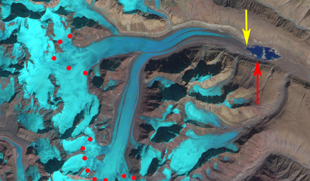
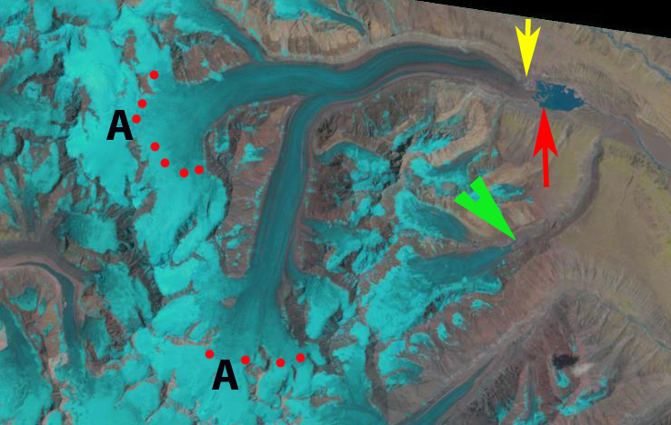
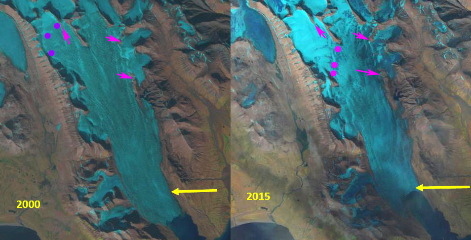
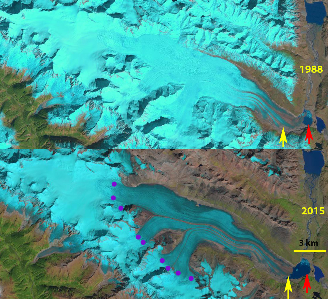
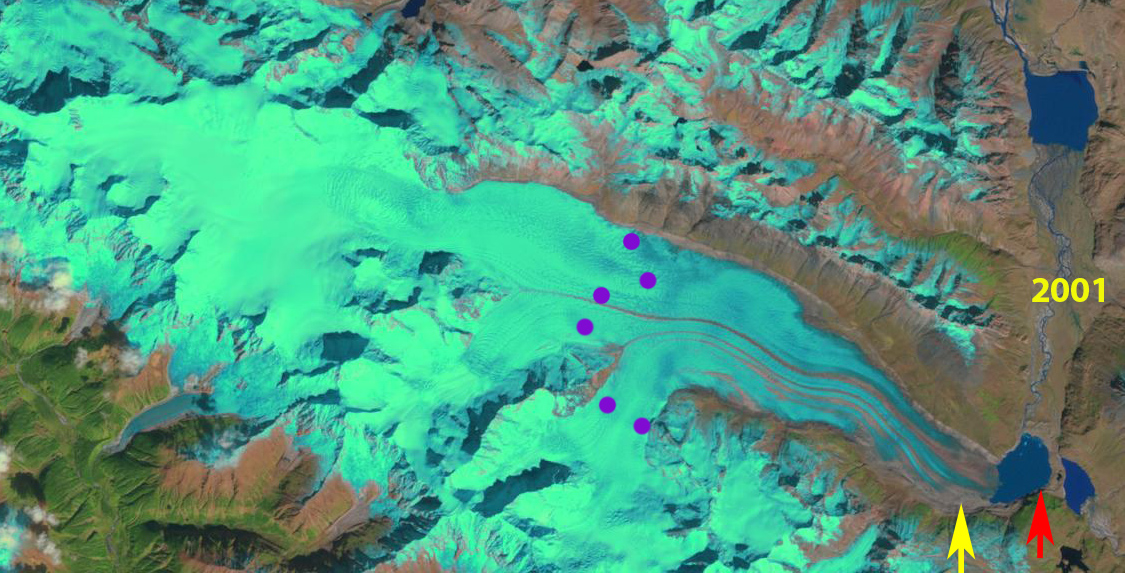
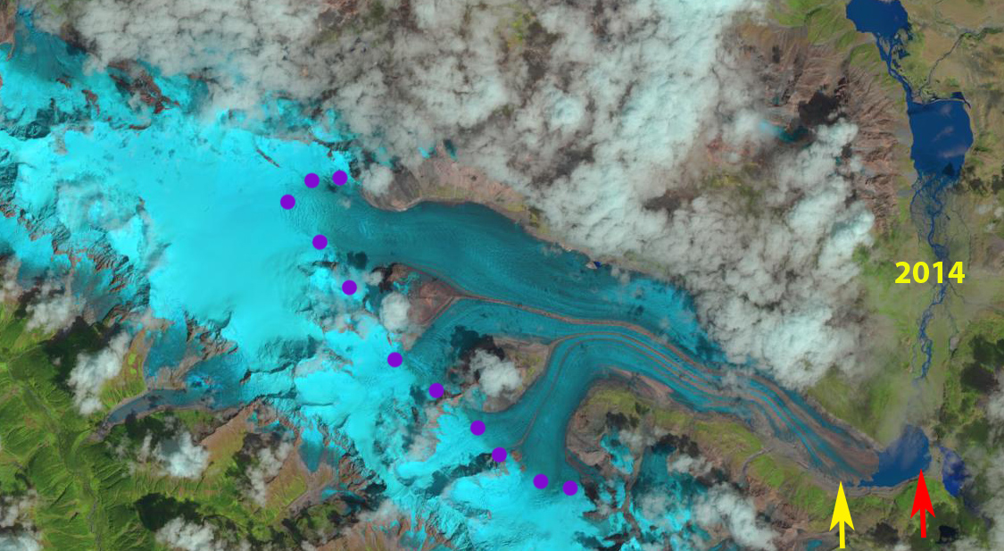
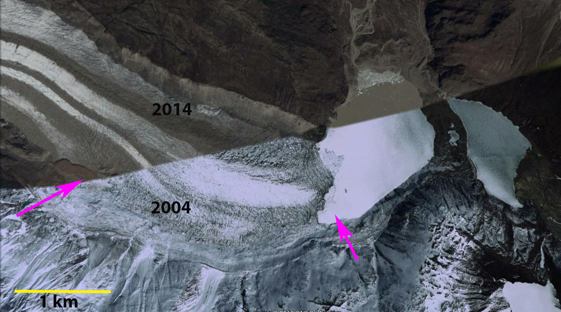
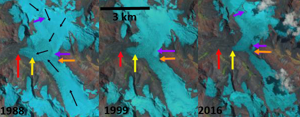
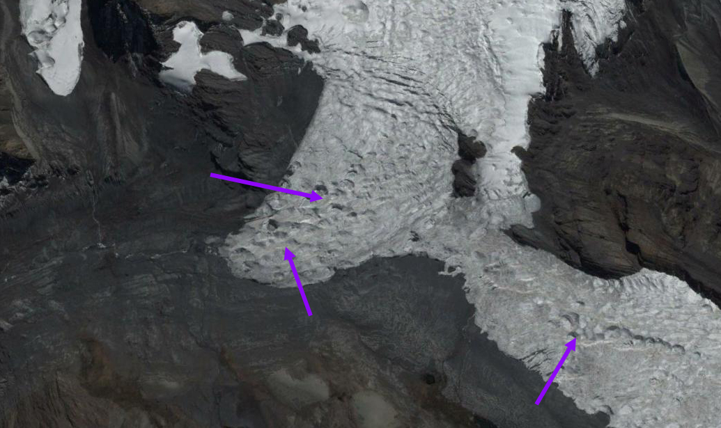
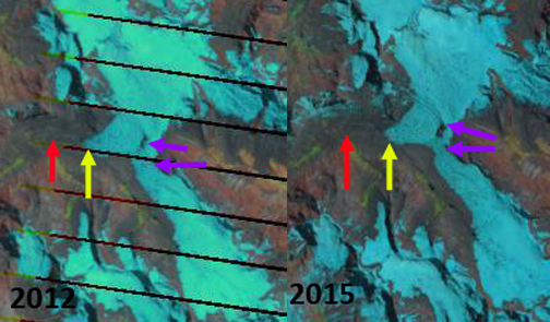
Figure 5. The Conrad Glacier terminus in 2014 (on the left) and 2016 (on the right). Between 2014 and 2016, the terminus of this glacier retreated by 75 m (yellow arrows) and the glacier also thinned markedly. The visibility of the rock band in the center of the image shows this thinning of the ice (red arrows). Also note the orbital crevasses (green arrow), which formed due to the collapse of ice caves along the margin. These ice caves formed in 2014 and 2015 as the surrounding exposed rock warmed (via solar heating) and melted the ice margins from below, and subsequently collapsed in 2016.

Spring arrived around four weeks earlier than normal this year, as we noted in our spring report, with the melt season commencing near the start of April instead of the start of May. At the beginning of April, the 2015-2016 winter had resulted in average snowpack in the northern half of the Columbia Basin and above-average snowpack in the southern half. However, early hot temperatures during April then led to early melt instead of a slow increase in snow throughout the rest of the spring. By mid-April, the snowpack across the entire basin had dropped to under 50% of the normal amount. One caveat here is that province-wide snow monitoring includes many measurements at around 2000 m, but very few above this elevation. Most glaciers in the Columbia Basin lie above 2000 m elevation, so our understanding of the snowpack affecting these glaciers is limited. While there are no long term records for higher elevations in the basin, our data, and discussions with local ski guides and lodge operators, suggests that the snowpack was probably around average during winter 2015-2016 until April.

Our measurements indicate that overall, the 2015-2016 winter resulted in a snowpack that was only 7% lower than the 2014-2015 winter. Why, then, was 2015 a year of substantial mass loss in the Columbia Basin but 2016 only a slightly negative year? The answer is that temperature difference has a far greater impact in this region than the amount of snow accumulation. In our region, at the elevation where glaciers are located (generally above 2000 m), the variability in snowfall year to year is far smaller than the variability in annual temperatures. Temperatures have risen over the Canadian portion of the Columbia River Basin by 1.5°C over the past century, more than double the global rate according to the Columbia Basin Trust. Due to rising temperatures, above-average snowpack is needed just to break even in a typical year. Thus, in order to have a positive mass balance year, you need above average snowfall and below average temperatures.

The summer of 2016 featured average to slightly above average temperatures (Figure 6), with a cooler-than-average July. This is in contrast to the last two years, which both featured well-above-average temperatures through the melt season. Precipitation was also about average over the basin during the summer months (Figure 7). The basin began with a roughly average alpine winter snowpack, experienced an early and hot spring, slightly warmer-than-average summer temperatures, and average precipitation. The combination of these factors led to a slightly negative mass balance overall for our glaciers in 2016: those in the north lost around 0.5 mwe and those in the south stayed around neutral or even slightly gained mass.

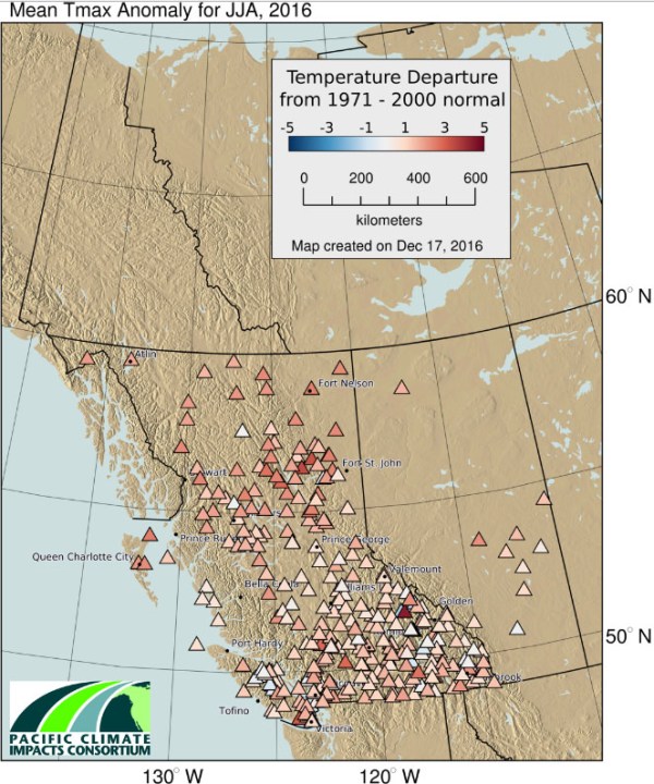
Figure 6. Summer (June/July/August) mean daily maximum temperature anomaly for British Columbia in 2016. The red ellipse highlights the Columbia Basin, where temperatures were average to slightly above average (data from the Pacific Climate Impacts Consortium).

The 2016 trend was likely due, in part, to the prevailing position of the jet stream in the 2015-2016 winter. The northerly position of the jet stream, and persistent ridge over the Pacific Northwest, led to warmer winter temperatures over the southern part of the Columbia Basin but also more moisture and concentrated storm tracks (calcification: while accumulation variability resulting from winter weather patterns may have played a role in the north-south trend, the magnitude of mass change (small loss) was controlled by melt season temperatures). My favorite location to observe the jet stream in winter is from the California Region Weather Server at San Francisco State University. There have been many discussions of the jet stream behavior and its influence on winter weather in this region (here’s a simple overview from NOAA). The north-south trend was observed in 2015 as well, but in reverse, with the glaciers in the south experiencing greater mass loss.

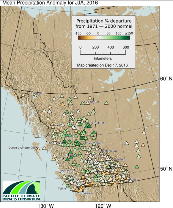
Figure 7. Summer (June/July/August) precipitation anomaly for BC. Red ellipse highlights the Columbia Basin. Columbia Basin precipitation was net average to slightly below average for summer 2016 (Pacific Climate Impacts Consortium).

Well-above-average snowfall and well-below-average spring, summer and fall temperatures would be needed for any of the Columbia Basin glaciers to gain substantial mass. This has happened just twice over the past 20 years, as recorded by the North Cascades Glacier Climate Program in the North Cascades of Washington, just southwest of the Columbia Basin. During the winter of 1999, Mt. Baker set the record for most snowfall ever recorded in the US at 1140 inches (or 2900 cm, yes…29 meters!), leading to average glacier mass gain of over 1 meter water equivalent (mwe). The winter of 2011 also featured above average snowpack, and in combination with a cool and cloudy summer, led to below-average melt and a positive mass gain of over 1 mwe. Unfortunately, closer to the Columbia Basin, the Peyto, Place and Helm Glaciers of British Columbia, have never reported a mass gain of 1 mwe since Geologic Survey of Canada records began for those glaciers in the 1960s and 1970s.

The take home points:

In 2016, glaciers in the Columbia Basin experienced a slightly negative mass balance year. There was slight mass gain in the south (less than +0.25 mwe) and moderate mass loss in the north (around -0.5 mwe).
At present, an average year still results in moderate glacier mass loss in the Columbia Basin. Either above-average snowpack or below-average temperatures are needed during the melt season for a neutral mass change. A combination of both is required for the glaciers to gain mass.

If you want to see what our fieldwork looks like in practice, see my video from the spring field season.

Samudra Tapu Glacier, India Accelerated Retreat 1998-2016

On December 26, 2016May 1, 2024 By mspeltoIn Himalaya glacier retreat

Landsat Comparison from 1998 and 2016 of Samudra Tapu Glacier, India. Red arrow is the 1998 terminus, yellow arrow the 2016 terminus, green arrow a subsidiary glacier tongue, red line and dots the snowline and pink arrow an area indicating a water level decline in the lake.

Samudra Tapu Glacier is one of the largest in the Chenab Basin, India. Maanya et al (2016) indicate the glacier terminates at 4150 m and is 16 km long and has an area of 62.5 square kilometers. In a glacier inventory in the basin by Kulkarni et al (2007) the 466 glaciers in the basin were observed to have lost 21% of their total area from 1962 to 2001. This study coordinated by the Space Applications Centre of the Indian Space Research Organization, has combined field observations of the glacier with remote sensing to observe the changes in area and length of the glaciers. The Chenab River also provides 690 MW of hydropower at the Salal Hydroelectric Project

In this post we use 1998, 2002 and 2016 Landsat imagery to examine the terminus of this glacier. The terminus in 1998 is in an expanding proglacial lake and the snowline is at 5200 m. In 2002 the glacier has retreated a short distance since 1998 and the snowline is at 5300 m. Note that the smaller glacier tongue at the green arrow is disappearing. An October 2016 image indicates a further lake expansion and a glacier retreat of 600 m since 1998. The lake level has also fallen as evident by the expansion of peninsula areas in the lake, pink arrow. A Sentinel 2 image from November 11, 2016 indicates the snowline is higher than in October or during the other years observed at 5400 m. The lower glacier is heavily debris covered, has a low slope and is essentially stagnant in its lowest 1 km, note image below from Anil Kulkarni. These factors will lead to continued retreat. There are some remarkably long supraglacial streams, the longest is 3.5 km long, that further illustrate the slow velocity of the lower glacier. This is in a region where ice thickness is 100-200 m, see image below Maanya et al (2016). Neither glacier is at the end of the melt season. The glacier at the green arrow has retreated well upvalley from the green arrow. This glacier is not calving into a lake and is retreating faster than Samudra Tapu. This suggests that the debris cover is reducing melting more than the lake is enhancing melting. In November 2016 the snowline is at 5400 m. An ELA of 5300+ meters leaves an accumulation area insufficient to maintain the current glacier size. In 1970 the ELA was at 4900 meters Kulkarni et al (2007) . The retreat of Samudra Tapu is noted by Kulkarni (2006) as 20 meters/year during the 1962-2000 period. From 1998 to 2016 the glacier retreated nearly 600 m, closer to 30 meters/year. The retreat of this glacier is less than that of other large glaciers nearby Sara Umaga and Gangotri, but similar to Durung Drung Glacier.

Sentinel 2 image from 11/11/16. Red arrow is the 1998 terminus, yellow arrow the 2016 terminus, red dots the snowline.

Landsat image from 2002. Red arrow is the 1998 terminus, yellow arrow the 2016 terminus, green arrow a subsidiary glacier tongue, red dots the snowline.

Image of the debris covered stagnant terminus of Samudra Tapu from Anil Kulkarni taken in 2006

The above figure is from Maanya et al (2016).

Has Fridtjovbreen, Svalbard Surged for the last time?

On December 20, 2016May 1, 2024 By mspeltoIn svalbard glacier retreat

Fidtjovbreen, Svalbard comparison in 1998 and 2016 Landsat imagery. Red arrow marks the 1998 terminus, yellow arrow the 2016 terminus and purple dots mark the snowline. The Yellow numbers indicate area of separation between glaciers. Pink arrows indicate areas on the upper glacier where thinning is exposing more bedrock. F=Fridtjovbreen, S=Sagabreen, G=Gronfjordbreen

Fridtjovbreen, Svalbard, is a tidewater-terminating glacier that started a 7-year surge advance during the 1990’s. This central Spitsbergen glacier drains into Van Mijenfjorden and is currently 13.5 km long. The glacier advanced ~2.8 km during a surge in the 1990’s at a maximum rate of ~4 m per day (Murray et al, 2003). Murray et al (2012) observed that from 1969 to 1990, the glacier retreated ~500 m and lost 5% of its volume. During this interval the glacier thinned up to 60 m in the lower elevations while thickening up to 20 m in its higher elevations. The upper part of the glacier is considered the reservoir zone, which after sufficient thickening and slope increase versus lower glacier glacier, receiving zone, surges yielding an increased flux into the receiving zone. If the reservoir zone is not an accumulation zone due to climate change, than the surge mechanism in this case is lost. Murray et al (2012) observed that the reservoir zone thinned by up to ~120 m and the receiving zone thickened by ~140 m during the most recent surge. Lonne et al (2014) examined glacial surges in Svalbard noting they are protracted and characterized by individual dynamic evolution. Fridtjovbreen provides a well documented example of a 12 year (1991–2002) surge. that Lonne et al (2014) report relocated 5 km2 of ice into the fjord, yet 15 years later leaves little visual evidence behind. The advance led to the overriding of Sagabreen (S) observed by Glasser et al (1998).

The most recent surge occurred in a climate of decreasing overall ice volume, but in an environment of accumulation zone thickening on Fridtjovbreen (Lonne et al 2014). Here we examine Landsat imagery that illustrates both retreat from 1998 to 2016 and that instead of thickening during the quiescent phase, high snow lines have led to thinning even at the head of the glacier. From 1998 to 2016 the glacier has retreated 2.2 km. This had led to separation from Sagabreen (1) from Fridtjovbreen. Thinning at higher elevations had led to bedrock expansion at each pink arrow in the comparison of 1998 and 2016, as well as the 2000 to 2015 imagery below. In each of the four years the snowline has risen to above 500 m by the end of the melt season. In 2016 the image is from the end of July, by early September the snowline had risen well above 500 m. There is also separation of glaciers adjacent to Gronfjordbreen at an elevation of 300 m, at Point 2 and 3. This implies that the reservoir zone is losing mass and cannot initiate a future surge. The thinning, retreat and volume loss parallels that of other glaciers in the area, that are not surging Frostisen and Paierbreen. Lonne et al (2014) note that although the surge mechanism itself is unrelated to climate, climatic conditions play a major role in the course of a surge. I would add that climate can eliminate the potential for a surge if the reservoir region is no longer an area of accumulation, without which there will not be thickening.

Fridtjovbreen, Svalbard comparison in 2002 and 2015 Landsat imagery. Yellow arrow the 2016 terminus and purple dots the snowline. Purple dots indicate the snowline and Pink arrows indicate areas on the upper glacier where thinning is exposing more bedrock.

Laigu Glacier, China Retreat Lake Expansion

On December 16, 2016May 1, 2024 By mspeltoIn china glacier retreat

Landsat image comparison of the Laigu Glacier in 1988 and 2015. The red arrow indicates the 1988 terminus and the yellow arrow the 2015 terminus location. The purple dots in 2015 indicate the snowline.

Laigu (Lhagu) Glacier, China is in the Kangri Karpo Mountains of the Southeast Tibet Plateau and drains into the Salween River. This is the largest glacier in its region at 32 km in length. The glacier terminates in an expanding proglacial lake, Laigu Lake. Here we examine changes in Landsat imagery from 1988 to 2015 to identify response to climate change. Wang and others (2011) note that glacial lakes have expanded from 1970-2009 by 19% and the area that is glacier covered has decline by 13% during the 1970-2009 period in the nearby Boshula Range. At the AGU this week research based on Landsat imagery indicates a 20% per decade velocity decline on the glacier (Landsat Science, 2016).

In 1988 Laigu Glacier terminated in the proglacial lake that was 2 km across from north to south and 1.3 km from east to west. By 2001 the lake had expanded to 1.6 km from east to west. The transient snow line is at 4300 m. In November, 2014 the snowline is at 4700 m. In October, 2015 the snowline is at 4700 m again. The glacier has retreated 1900 m from its 1988 terminus along the southern shore of the expanding lake and 900 m along the northern shore. The expansion of the lake along the southern shore is evident in the 2004 and 2014 Google Earth segmented image below, note the pink arrows. The high snowline indicate a reduced accumulation, which reduces the flux into the ablation zone, this is evident in the reduced glacier velocity noted by Dehecq (2016). The reduced velocity will lead to a continued retreat of the glacier and expansion of the lake. This region has experienced a sustained rise in summer temperatures (Wang and others, 2011). The snowlines remaining high into November indicates warmer conditions in the post summer monsoon season also. The high snowlines and lake expansion due to glacier retreat is a familar story in the region, Chutanjima Glacier and Menlung Glacier.

Landsat image comparison of the Laigu Glacier in 2001. The red arrow indicates the 1988 terminus and the yellow arrow the 2015 terminus location. The purple dots in 2001 indicate the snowline.

Landsat image comparison of the Laigu Glacier in 2014. The red arrow indicates the 1988 terminus and the yellow arrow the 2015 terminus location. The purple dots in 2014 indicate the snowline.

Google Earth image of the region indicating the lake expanding from the pink arrow at right to the pink arrow at left from 2004 to 2014.

Summer temperature rise form Wang and others (2011).

Norrearm Fjord Glacier Retreat, Greenland

On December 9, 2016May 1, 2024 By mspeltoIn glacier climate change, Glacier Observations, Greenland glacier retreat

Apostelens Glacier in Norrearm Fjord Landsat comparison from 1999 to 2016. Red arrows are the 1999 terminus location, yellow arrows the 2016 terminus location and purple arrows indicate an expanding bedrock ridge.

“Apostelens” Glacier drains east from a peak of the same name into an arm of Norrearm Fjord, which in turn is part of Lindenow Fjord in southern Greenland. The glacier is a short distance north of Kangersuneq Qingordleq, where recent retreat has led to glacier separation. The glacier is soon to lose its tidewater connection as has occurred at Tasermiut Fjord to the west. This will result in a decline in iceberg production as well.

Here we examine Landsat imagery from 1999-2016 to identify glacier change. In 1999 the Apostelens arm of Norrearm Fjord is largely filled by the glacier which extends to within 2.5 km of Norrearm Fjord, red arrow. The tongue contains numerous ogives formed each year due to seasonal velocity changes through an icefall. This is evident in the Google Earth image from 2004, where 24 ogives are evident on the low slope glacier tongue, in 1999 the number is over 30. By 2013 the glacier has retreated nearly 2 km from the 1999 terminus position, red arrow. In 2012 Google Earth imagery indicates increased crevassing near the front and the loss of most ogives. New ogive formation is also hard to distinguish. By 2016 the glacier has retreated 2.6 km and is nearing the headward limit of the fjord arm. The collapse of the fjord tongue and its associated ogives indicates the loss of 30 years worth of volume flux that emerged from the icefall that generated the ogives.

Greenland tidewater outlet glaciers in this region have experienced substantial retreat since 1990, Weidick et al (2012) and Howat and Eddy (2011). Murray et al (2015) examined 199 tidewater glaciers in Greenland and noted significant retreat of 188 of them. Apostelens Glacier was not one of these, and soon will not be a tidewater glacier to be included in the list.

Apostelens Glacier in Norrearm Fjord Google Earth comparison from 2004 and 2012. Red arrows are the 2004 terminus location, and yellow arrows the 2012 terminus location. Note ogives in 2004 and loss of them in 2012.

Map of the Norrearm Fjord region and Apostelens Glacier, with blue arrows indicating flow.

Nevado Soral, Bolivia Glacier Retreat Separation Imminent 1988-2016

On December 5, 2016May 1, 2024 By mspeltoIn bolivia glacier retreat

Landsat comparison from 1988 to 2016 of Nevado Soral Glaciers, Bolivia. Red arrow is the 1988 terminus, yellow arrow the 2016 terminus, orange arrow is the glacier junction and the purple arrow areas of rock expansion indicating upglacier thinning.

Nevado Soral is in the Cordillera Apolobamba Range of the Bolivian Andes. A significant valley glacier flows south from the mountain joining a northward flowing glacier shortly above the terminus. The combined runoff of these glaciers drains in to Laguna Suches, which is transected by the Bolivia-Peru Border. Cook et al (2016) quantify the importance of the Bolivian Andes Glaciers for water supply for Andean cities and mountain communities. They used Landsat satellite imagery to identify an overall areal shrinkage of 228 km2 (43%) across the Bolivian Cordillera Oriental between 1986 and 2014, including 43% in the Cordillera Apolobamba, where Nevado Soral is located. Retreat has led to a growing number of lakes, although the number of ice-contact lakes has decreased. Vuille et al (2008) noted that air temperature in the Andes has increased by approximately 0.1 °C/decade, with only two of the last 20 years being below the 1961–90 average. Soruco et al 2009) observed glacier change in the Cordillera Real of Bolivia and determined that between 1963 and 2006 the mass of these glaciers has clearly been decreasing since 1975 without any significant acceleration of this trend over recent years. The net result was that glaciers lost 43% of their volume between 1975 and 2006. On nearby Chaupi Orko Glacier retreat has been less extensive, but several new lakes have formed in the last two decades.

In 1988 the junction where the north and south flowing glacier meet and turn west is 800 m wide, orange arrow. The main glacier terminus is at m, red arrow. The purple arrows indicate areas where no bedrock is exposed. In 1999 there is 250-300 m of retreat and bedrock is still not exposed at the purple arrows. By 2016 the main terminus has retreated 800 m since 1988. The junction of the glacier is only 300 m wide. The purple arrows indicate locations where bedrock has been exposed by glacier thinning. A Google Earth closeup below indicates significant ablation hollows, and few surface streams, suggesting that sublimation is an important means of ablation on the glacier. The narrow junction of the two glaciers will soon melt, leaving two separate glaciers.

Terminus zone of Nevado Soral Glacier. Purple arrows indicate ablation hollows are as common as stream channels. This typifies an area where sublimation is a significant source of ablation.

Landsat comparison from 2012 and 2015 of Nevado Soral Glaciers, Bolivia. Red arrow is the 1988 terminus, yellow arrow the 2016 terminus and the purple arrow areas of rock expansion indicating upglacier thinning.

Nevado Soral Glacier drains into Laguna Suches.

Semienova Glacier, Kyrgyzstan Area, Volume, Velocity Decline

On December 1, 2016May 1, 2024 By mspeltoIn tien shan glacier retreat

Landsat comparison of Semenova Glacier in 1998 and 2016. Red arrow is the 1998 terminus, yellow arrow is the 2016 terminus and purple are locations where tributaries are separating from each other or disconnecting from the main glacier.

Semienova Glacier is a valley glacier in the northeast corner of Kyrgyzstan draining into the Sary Dzhaz (Aksu) River which then flows into the Tarim Basin, China. Farinotti et al. (2015) used three approaches to assess glacier change in the Tien Shan from 1961 to 2012. The results converge on an overall loss of glacier area of 19-27%,a glacier spatial extent of 2960 square kilometers. They further observed that it is primarily summer melting that has driven the change. Sorg et al (2012) showed that glacier shrinkage is most pronounced in peripheral, lower-elevation ranges near the densely populated regions, where summers are dry and where snow and glacial meltwater is essential for water availability. Shifts of seasonal runoff maximum have already been observed in some rivers, and further summer runoff reductions are expected. Li et al (2014) identify a reduction in velocity of a number of large glaciers, including Semienova Glacier in the Tien Shan from 2007-2011 that is likely due to mass losses. Semienova Glacier had a peak velocity 10 km above terminus at 12 cm/day, declining to less than 2 cm day in the last 1-2 kilometers.

From 1998 to 2016 the glacier has retreated 500 m, this is a relatively modest retreat for a glacier of this size. Debris cover has expanded and supraglacial stream networks have expanded indicating an increasingly stagnant terminus tongue, supporting the low velocity observations. There are three tributaries that joined the glacier in 1998, at the 3 eastern most purple arrows, have detached from the main glacier by 2016. This indicates reduced contributions to the main glacier tongue. The two purple arrows on glaciers flowing into the valley from the south are located where two formerly joined glaciers are increasingly separated. The snowline in the glacier separating the melt zone and accumulation zone was at 4000 m in 2002, 2013 and 2016. The retreat of glaciers in the region has also been observed in the Barskoon Mountains and Petrov Glacier.

Sentinel image of Semienova Glacier in 2016. Black arrow is 1998 terminus, white arrow the 2016 terminus and black dots the snowline in 2016.

Landsat images of Semenova Glacier in 2002 above and 2013 below. Red arrow is the 1998 terminus, yellow arrow is the 2016 terminus and purple are locations where tributaries are separating from each other or disconnecting from the main glacier. Purple dots indicate the snowline.

Hornopirén Glaciers, Chile in Spectacular Retreat

On November 28, 2016May 1, 2024 By mspeltoIn chile glacier melt, chile glacier retreat

Landsat comparison of Rio Blanca Glaciers in Hornopirén National Park, Chile from 1985 to 2016. Red arrow 1985 terminus, yellow arrow 2016 terminus, purple dots the snowline and purple arrows expanding bedrock areas amidst the glacier.

Hornopirén National Park is in the Los Lagos region of Chile. The park is host to a number of glaciers that are in rapid retreat. Davies and Glasser (2012) mapped the area of these glaciers with 113 square kilometers in 1986 and 96 square kilometers in 2011. The retreat of the largest glaciers in the park is nothing short of spectacular in recent years. Here we examine Landsat imagery to identify changes in two or the larger valley glaciers from 1985-2016. These glaciers from the headwaters of the Rio Blanco and are designated Rio Blanco North (RBN) and Rio Blanco South (RBS). Rio Blanco enters the ocean just east of the community of Hornopirén.

In 1985 the two glaciers merged just before the western terminus of the icefield at 820 m, red arrow. The snowline was at 1300 m. There is also an eastern outlet of RBN, terminating at the north end of a basin, red arrow. By 1998 RBN and RBS had separated by over 1 km with the formation of a new lake at the former terminus. The eastern terminus of RBN has begun retreat and is now ending in a proglacial lake. RBS is developing a nunatak at the purple arrow. The snowline was again near 1300 m. By 2016 RBN has retreated 4.5 km, and now terminates at 1200 m, yellow arrow. The deglaciated valley now hosts three alpine lakes that did not exist in 1985. The eastern terminus of RBN has retreated 1100 m and is still terminating in an expanding alpine lake, yellow arrow. By 2016 RBS had retreated 3.4 km since 1985, terminating at 1180 m, yellow arrow. The nunatak in the lower section of RBS, purple arrow, has continued to expand. RBN has lost 56% of its length since 1985 and RBS 37% of its length.The snowline in 2015 and 2016 is at 1600-1700 m. This leaves only a small percentage of the glacier area above the snowline. The large valley glaciers that just 30 years dominated the headwaters of Rio Blanco have lost much or their area and will soon be small slope glaciers clinging to the highest peaks. Retreat here is more extensive than seen 100 km to the northwest at Calbuco Volcano and for the Northern Patagonia Icefield.

Landsat comparison of Rio Blanca Glaciers in Hornopirén National Park, CVhile from 1998 to 2015. Red arrow 1985 terminus, purple dots the snowline and purple arrows expanding bedrock areas amidst the glacier.

East Terminus of Rio Blanca North, with the newly formed lake. This terminus is above 1300 m and has retreated largely via iceberg calving.

RG150-17.01019 Glacier Retreat, Southern Patagonia Forms Lake

On November 21, 2016May 1, 2024 By mspeltoIn chile glacier melt, chile glacier retreat

Retreat of RG150 indicated in Landsat images from 1984, 2001 and 2015. Red arrow indicates 1984 terminus and yellow arrow 2015 terminus.

RG150 is a 3.5 km long glacier in Bernardo O’Higgins National Park on the western edge of the Southern Patagonia Icefield, Chile. RG150 is an unnamed glacier given this designation as part of the Randolph Glacier Inventory. The glacier terminates in a lake that drains into Seno Andrew. Willis et al (2012) observed that between February 2000 and March 2012 that the Southern Patagonia Icefield is rapidly losing volume and that thinning extends even to high elevations. The mass balance loss is occurring at a rate of −20.0 ± Gt/year, which is +0.055 mm/year of sea level rise. The retreat has been driven by increasing calving rates from the 1975-2000 to the 2000-10 period (Schaefer et al, 2015). The pattern of retreat is consistent between these glaciers and the region as noted by Davies and Glasser (2012), annual rates of shrinkage in the Patagonian Andes increased in from 0.10% year from 1870-1986, 0.14% year from 1986-2001, and 0.22% year from 2001-2011. Davies and Glasser (2012), note the all the glaciers in the complex inclusive of RG150 had their fastest retreat period from 2001-2015. Glasser et al (2016) observed both an increase in glacier proximal lakes and in debris cover on glaciers with glacier retreat from 1987-2015. These losses have led to retreat such as at Balmaceda Glacier, Glaciar Marconi and Glacier Onelli. Here we examine Landsat imagery from 1984 to 2015 to identify glacier change and the formation of a new lake.

In 1984 there was no glacier lake at the terminus, with the lower 1 km of the glacier being a low sloped glacier tongue. By 2001 a small proglacial lake had developed 250-300 m long. In 2005 the glacier retreat had led to continued lake expansion. The glacier had filled the lake with numerous small icebergs. By 2015 the glacier still terminates in the proglacial lake that is not 850-900 m long. The glacier retreat of 850 m since 1984 is 20-25% of the total glacier length. The low slope region is minimal in length in 2015 indicating the lake basin is almost complete. This will lead to a reduced rate of retreat. This is a very cloudy region, and the images here are not at the end of the melt season. Hence, the equilibrium line altitude can be ascertained. At the crest of the glacier 1300 m, there are a number of wind sculpted features that are 400-600 m long, attesting to the strong westerly winds in the region. RG150 has significant retained accumulation each year and can survive the current climate.

Retreat of RG150 indicated in Google Earth images from 2005 and 2015. Red arrow indicates 1984 terminus and purple arrows indicate wind features at the top of the glacier.

RG150 in Google Earth image looking upglacier in 2015. Red arrow indicates 1984 terminus and yellow arrow 2015 terminus and purple arrows indicate wind features at the top of the glacier.

Barnes Ice Cap, Baffin Island Evident Response to Climate Change

On November 18, 2016May 1, 2024 By mspeltoIn Canada glacier retreat1 Comment

Barnes Ice Cap transect and closeup of divide area in August 2016. Black dots indicate summit divide of the ice cap. Notice the channels extending away from the divide. These are not stream channels, as they are too wide, but they are meltwater formed valleys that are preferred pathways for the meltwater transport.

Barnes Ice Cap located in the center of Bafﬁn Island, Canada covers an area of ~5800 km2. The ice cap is approximately 150 km long, 60 km wide and has maximum ice thickness of ~730 m and a maximum ice elevation of 1124 m above sea level (asl) at the summit of the north dome (Andrews, 2002). They also note a retreat of the southeast margin of 4 m/year from 1961-1993 on the southeast margin (Jacobs et al 1997). Dupont et al (2012) identified that the melt season increased from 66 days fro the 1979-87 period to 87 days from 2002-2010. They also noted that ICESat altimeter data indicated the thinning of the BIC at a mean rate of 0.75 m/year for the 2003–2009 period. Gilbert et al (2016) Figure 5 indicates the ELA was at 950 in the 1960-80 period and is at 1100 m from 2002-2010 this leaves a limited accumulation zone area. observe that Barnes Ice Cap has nearly lost its accumulation area over the last 10 years, in part due to the longer melt season. The glacier does tend to not retain snowcover the accumulation zone consists of superimposed ice at the crest. Papasodoro et al (2016) noted that glacier wide balances were −0.52 m w.e./year from 1960 to 2013 and doubled to −1.06m w.e./year from 2005 to 2013. They also The drainage channel development suggests meltwater transport from versus refreezing of meltwater in 2016.

Landsat comparison of the northwest margin of the Barnes Ice Cap in 1990 and 2016. Red arrows indicate terminus locations in 1990. Purple arrows indicate an area of stream development parallel to the ice front. The bright area at the margin of the ice cap is Pleistocene ice (Andrews, 2002).

Here we examined Landsat imagery from 1990-2016 to illustrate the retreat of the northwest region of the icecap and to take a look at the 2016 melt features and lack of any retained snowcover on the ice cap. In 2016 the melt channels from the divide at the crest of the ice cap are impressive. There is no retained snowcover at the summit of the ice cap even on August 9th with several week left in the melt season. The melt pathways visible in the imagery from 2016 extend 10 km downslope from the crest of the icecap. In 1990 the ice cap terminated at the red arrows, this included contact with a peninsula in Nivlalis Lake and an island in Conn Lake. By 2011 and 2014 the glacier had retreated from the locations. In 2016 the total retreat of the margin has been 600 m at Nivalis Lake, 1100 m at the island in Conn Lake and 450 m further east at the red arrow halfway to Bieler Lake. This is a slow retreat rate compared to many glaciers, but represents a much higher rate than before 1990, with rates of 18-42 m/year. There is a new section of river parallel to the ice cap margin between Conn and Bieler Laker.

2011 Landsat image of northern margin indicating retreat from the 1990 postiion red arrows.

2014 Landsat image of northern margin indicating retreat from the 1990 postiion red arrows.

Hagafellsjokull, Iceland Reflects Langjokull Thinning & Retreat

On November 14, 2016May 1, 2024 By mspeltoIn glacier climate change, Glacier Observations, iceland glacier retreat

Landsat comparison of the terminus of Hagafellsjökull from 2000 and 2016. The red arrows are the 2000 terminus, the yellow arrows the 2016 terminus. Purple arrows indicate upglacier thinning.

Langjökull is the second largest iceap in Icalnd with an area of over 900 square kilometers. The mass balance of the icecap has been reported since 1997 and his lost over 1 m per year during this period (WGMS, 2016). Pope et al (2010) noted that the icecap has lost an area of 3.4 ± 2.5 km2 yr-1 over the decade from 1997-2007. Pope et al (2010) noted that the loss of ice volume confirms previously published predictions that Langjökull will likely disappear within the next 200 years if current trends continue. A key outlet of Langjökull is Hagafellsjökull which terminates in Hagvatn. Hagafellsjökull ended a sustained post Little Ice Age retreat in 1970. The ensuing advance of approximately 1 km ended by 2000. Here we examine Landsat imagery from 2000-2016 to identify recent changes in this outlet glacier.

In 2000 the glacier terminated on an island in Hagavatn, red arrow. The east margin of the glacier featured several locations where secondary termini overflowed a low ridge on the east side of the glacier. By 2006 the glacier had retreated 500-600 m from the island. By 2016 the terminus had retreated across its entire width by 800-850 m, 50 m/year, yellow arrows. A closeup view from the Iceland online map application illustrates the 2014 terminus red dots. The end of the glacier has a low slope, low velocity and is debris covered. The western side has terminated on land during this entire period and has approximately the same retreat rate as the eastern half that still ends in the expanding lake. There is little evidence of iceberg release into the lake, which helps explain the similar retreat rate. The low slope and upglacier thinning noted at the purple arrows indicate the retreat will continue. In 2014 the transient snowline reached near the head of the glacier at over 1100 m. In 2000, 2006 and 2016 the snowline with several weeks left in melt season ranged from 859-950 m. The retreat is similar to that of Norðurjökull another outlet of the Langjökull and Porisjokull.